Document Actions
gvSIG-Desktop 1.10. User Manual
- Analisys and procesing data
- Vectorial
- Geoprocessing tools
- Introduction
- Accessing the geoprocesses
- Buffer
- Intersection
- Clipping
- Dissolve
- Merge
- Convex hull
- Difference
- Union
- Spatial join
- 2D Translation
- Reprojection
- Exporting layers
- Introduction
- Exporting a shape
- Exporting to dxf
- Exporting to postgis and Oracle Spatial
- Exporting to gml
- Exportar a kml
- Annotation layer
- Introduction
- Creating an annotation layer
- Editing an annotation layer
- Annotation layer properties
- Adding an annotation layer to the view
- Example of how to create an annotation layer
- Export to a raster layer
- Crear shape de geometrías derivadas
- Raster
- Layer functionalities
- Filters
- Histogram
- Radiometric enhancement
- Save View as image
- Clipping layers
- Zoom to raster resolution
- Automatic vectorization
- Analysis view
- Geographic Transformations
- Alphanumeric
Analisys and procesing data
Vectorial
Geoprocessing tools
Introduction
The gvSIG geoprocessing extension allows you to apply a series of standard processes to the vector information layers loaded in the layer tree in a gvSIG view (ToC), thus creating new vector information layers which will provide new information for the source layers.
The following geoprocesses have been implemented in the first version of the geoprocessing extension:
- Buffer.
- Clip.
- Dissolve (by adjacents and alphanumerical criteria).
- Merge
- Intersection.
- Join.
- Spatial Join.
- Convex Hull (minimum convex polygon).
- Difference.
The output layer can take one of the output formats supported by gvSIG (it can only be saved in shp format at the moment).
When some geoprocessing tools are applied (for example, Clip) a window appears in which a spatial index can be created for the input layer. This is an internal process which is only carried out once per layer and per new project and speeds up the spatial intersection processes.

To create a spatial index for the input layer which can be used by the geoprocesses, click on “Yes”.
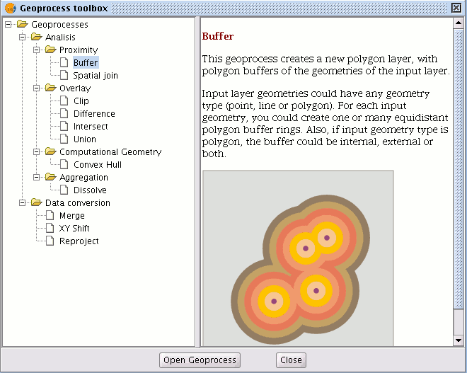
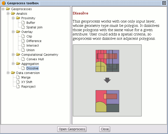
Accessing the geoprocesses
You can run the geoprocesses available in gvSIG with the geoprocessing wizard by clicking on the following tool bar button:

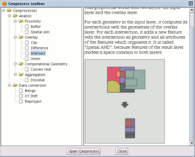
The “Geoprocess toolbox” will appear and you can use it to select the geoprocess you require. To access the different geoprocesses, pull down the tree in the window shown below (double click with the left button of the mouse on the "Geoprocesses" folder and the rest of the folders will appear).

When you have found the geoprocess you wish to use, click on the “Open geoprocess” button.

Buffer
Introduction
This geoprocess generates “areas of influence” around the vector element geometries (points, lines and polygons) of an “input layer”, thus creating a new polygon vector layer.
Several equidistant concentric radial rings can be generated around the input geometries. Moreover, in the case of polygon input geometries, the area of influence can be outside the polygon, inside the polygon or both inside and outside it. Some examples of the creation of areas of influence include:
- Which urban areas lack schools in a 1000m radius.
- Which wells do not comply with regulations on observing the minimum distance between two consecutive wells.
- River bed flood zones to monitor flood risks.
Creating an area of influence or buffer
When you click on the “Geoprocessing wizard” button, the following dialogue appears:
If you select “Buffer” and click on the “Open geoprocess” button, the window associated with this process is shown:
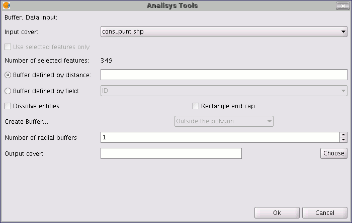
The form is divided into the following parts:

Selecting the elements whose buffer is to be computed. This is a pull-down list in which you can select the vector layer the calculation is to be applied to. If you wish, you can enable the “Use selected features only” check box so that the process only computes the buffer of the elements currently selected in the specified layer.
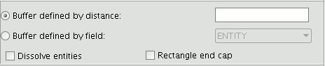
Inputting the features of the buffer to be computed. You can choose to input the buffer defined by distance (in the first text box) or to input a field in the input layer, from which the buffer radius value to be applied will be taken. This second option allows you to apply different buffer radii to different vector elements (whilst the first option applies the same radius to all the elements in the input layer). When the buffer of all the input layer elements has been generated, the “Dissolve features” option allows you to merge the elements whose geometries touch each other in a second iteration.
The “Rectangle end cap" option allows you to generate buffers with perpendicular edges (not rounded). Selecting the number of concentric buffers and their situation regarding the original geometry. The gvSIG “Buffer” geoprocess allows you to generate several equidistant areas of influence of the original geometry (for example, if the buffer distance to be applied is 200m and you choose to generate two concentric radial rings, the buffer distance of the second ring will be between 200-400m. Currently, you can only generate a maximum of three concentric radial buffer rings for efficiency reasons. If the vector layer we are working on is a polygon layer, the “Create Buffer…” option will be enabled, thus allowing the user to generate buffers outside, inside and both inside and outside the original polygon.

Introducing the result layer characteristics. Currently, the result of running a geoprocess can only be saved as an shp file. Thus, gvSIG allows you to select an existing shp file to overwrite it or to specify a new one. As new formats are supported to save the result of the geoprocesses, wizards will be provided to indicate the characteristics of these formats.

When you have input all the necessary information to compute the buffer, and clicked on the “Ok” button, a check routine is carried out to ensure that the information input is correct: whether the radius distance is numerical, whether the attribute from which the buffer radii are taken are numerical, whether a result file has been input, etc. If the check routine is not correct, a dialogue box appears so that the input data can be corrected.
If the input information that you have entered is correct, a window with a progress bar appears, in which the buffer processing rate is shown.
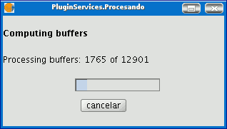
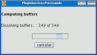
The process can be cancelled at any time by clicking on the “Cancel” button. As a consequence, the result file and any other intermediate product generated as a result of running the process are deleted. Whilst the buffer computing process is underway, other tasks can be carried out, such as changing the zoom or adding new layers to the layer tree in the gvSIG view. Other tasks can be carried out because all the geoprocessing extension geoprocesses are run in the background. When the process has finished, the new result layer is added to the layer tree in the active view. It is made up of buffer polygons with a specified radius based on the source layer.
Finally, the “Dissolve elements” option can be useful in specific situations (such as when the aim of computing the buffer polygons is to determine the total surface area affected by a phenomenon: quarantine areas, etc.), because when the generated polygons are merged the surface area covered by the buffer will be a real surface area, i.e. the sum of two buffers will not have any overlays.
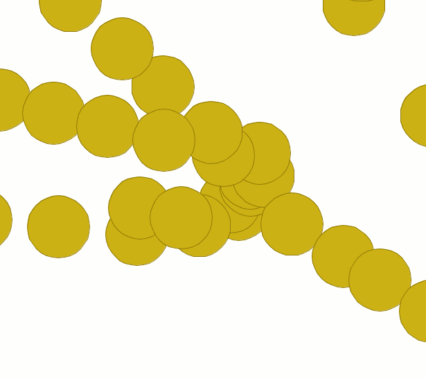
The above image shows non-merged overlay polygons. The total area covered by the phenomenon does not coincide with the sum of the individual areas.
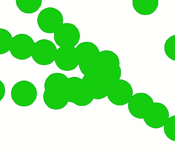
However, this second image shows merged overlay polygons. The total area covered by the phenomenon is real. When the buffer computing process includes the merger of overlay areas (dissolve) we cannot predict its exact duration (we do not know how many polygons will touch each other a priori). This is why the gvSIG geoprocessing extension does not show us a progress bar as such, it shows us a bar which periodically reaches the end and then goes back to the beginning. This type of process is called an “indeterminate” process.
Intersection
Introduction
This geoprocess operates on two layers, the “input layer” and the “overlay layer”, whose geometries can be polygons, lines or points.
It calculates the intersection with the different geometries in the “overlay layer” for each geometry in the “input layer”, thus creating a new element for each intersection. This element will take all the alphanumerical attributes in the geometries that created it (input and overlay). This is why (it models space areas which comply with the condition of belonging to the two polygons, lines or points that created it) this geoprocess is known as “Spatial AND" operator.
An example of how this geoprocess can be applied:
Given a land use layer (e.g. Corine2000), and a national geological map layer, you can obtain a polygon layer with homogeneous information on land use and geological material.
Running the 'Intersection' geoprocess
After selecting the "Intersection" geoprocess, the following dialogue appears:
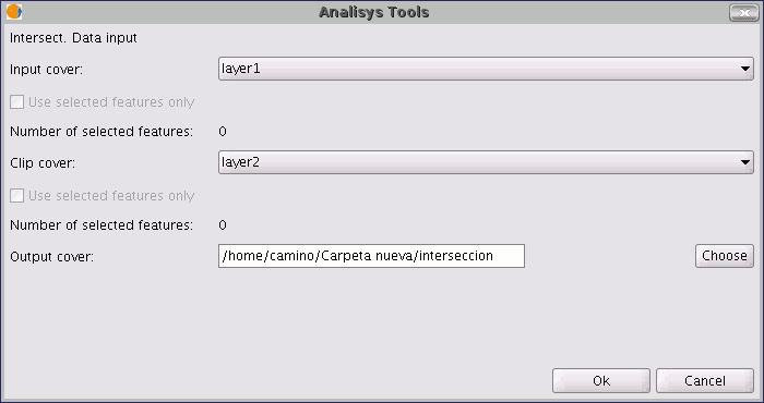
Select the input layer and the overlay layer. You must also specify a file in which to save the results. Finally, click on "Ok" and the geoprocess will be run.
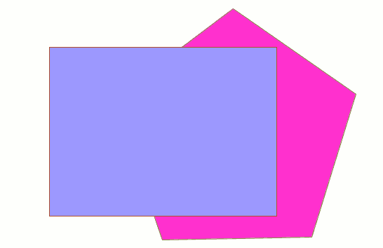
In this case, we will use a very simple example to better understand the function of the geoprocess. The previous figure shows two overlaying polygons. The result of launching the “Intersection” geoprocess with these layers as parameters is as follows:
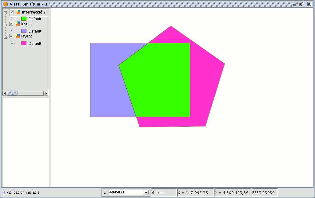
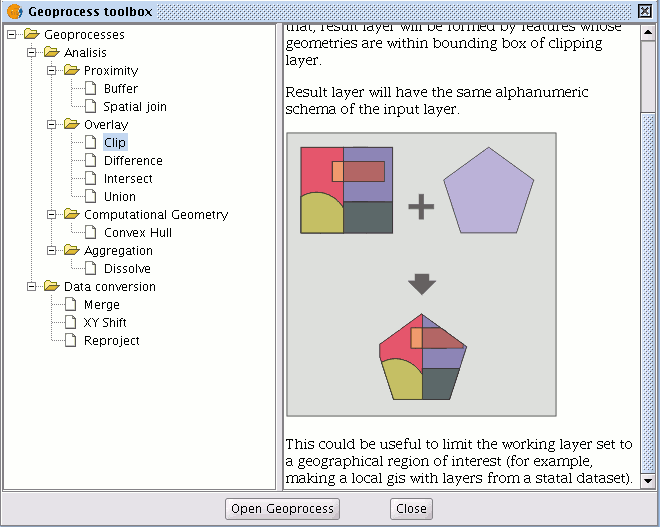
Clipping
Introduction
This geoprocess allows you to limit the working area of a vector layer (points, lines or polygons), and to extract an area of interest from it.
To do so, you need an “input layer” (the layer you will use to extract an area) and a “clipping layer” so that the union of the geometries included in the "clipping layer" defines the working area.
The geoprocess checks all the vector elements in the “input layer” and will calculate the intersections for the vector elements contained in the working area defined by the “clipping layer”, so that in the "result layer" only the vector elements of our working area will appear. The geometry portion that lies outside the working area will be clipped. The alphanumeric schema of the input layer remains intact.
Examples of use:
Setting up a local GIS would allow you to include national or regional maps and then to delimit the city or town as the working area.
Running the Clipping geoprocess
When the "Clip" geoprocess has been selected, the following dialogue appears.
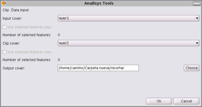
This dialogue allows you to select which layer you wish to clip, and gives you the chance to only clip the elements which are selected in the layer.
It allows you to select which layer will be used as the clipping layer and whether you wish to use the union of all the polygons in the clipping layer as the clipping polygon or just the selected elements.
Finally, as in the case of the other geoprocesses in gvSIG's geoprocessing extension, you can define how the result layer will be saved (at present you can only save it as a shp file).
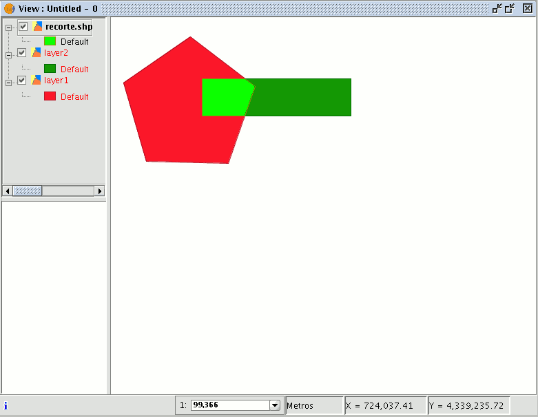
As a result of running the geoprocess, you will have a new layer in which only the geometries which came under the union of the clipping geometries have been kept.
Dissolve
Disolve
This geoprocess only acts on one “input layer”. The process analyses each entity in the "input layer" and merges the elements that have an identical value for a specific field into one element. Moreover, it allows you to involve spatial criteria in the decision to merge several features. This allows you to establish that for two elements to be merged, they must be adjacent to each other in addition to having the same value in the specified attribute.
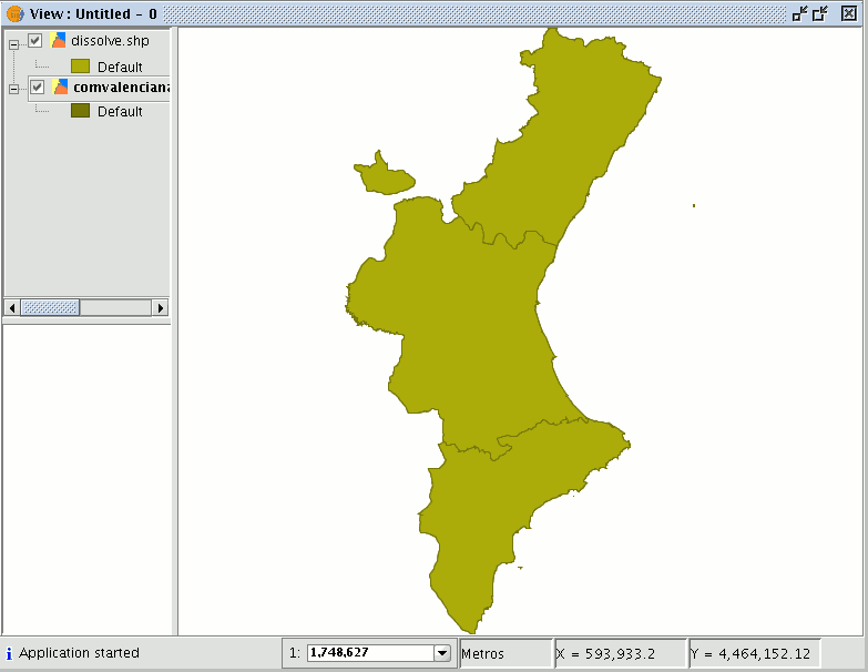
Example: We have a polygon layer which represents the municipalities of a particular autonomous region and we need a polygon layer with the provinces which make up this region. We can generate a province layer by launching the “Dissolve” geoprocess and specifying that the polygons that have the same value for the "PROV" field in which a unique code for the province is specified are merged.
Running the 'Dissolve' geoprocess
Using the previous example, we start by taking a "local layer" which we wish to convert into a "provincial layer".
When the "Dissolve" geoprocess has been selected, the following window appears:
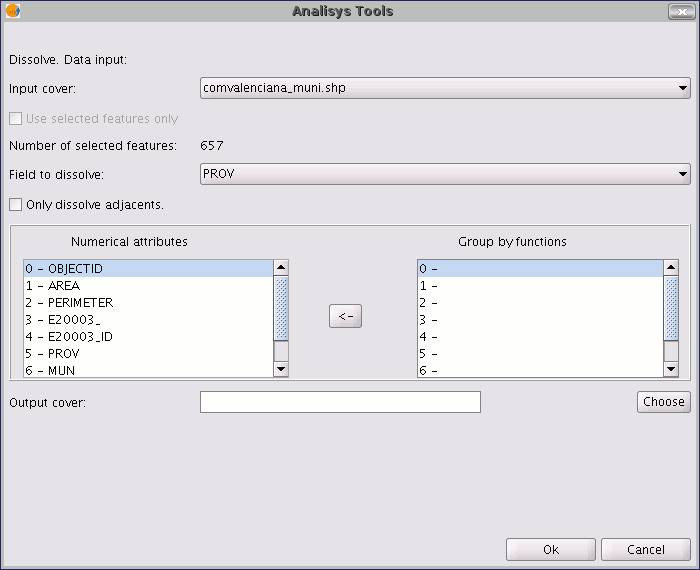
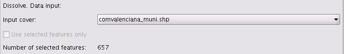
Firstly, select the layer you wish to dissolve (you can only work with a selection of elements in this layer).
You then need to specify the attribute of this layer which is going to be used as the criterion to merge the adjacent polygons. In our example, we must choose the “PROV” attribute.
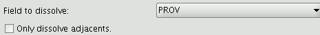
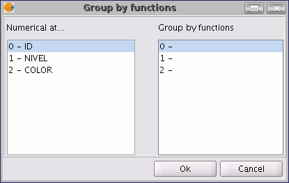
The polygons to be merged must have the same value for the dissolving attribute and in addition, you can choose whether they are adjacent to each other (spatial criteria). If you wish to choose this option, enable the "Only dissolve adjacents" check box. The gvSIG geoprocessing module allows you to keep a summary of the input layer polygon attributes once they have been merged. To do so, the “Summary function” concept is introduced. As each polygon of the “Dissolve” geoprocess result layer is the product of joining several input layer polygons, a summary function on the numerical attributes of the merged polygons can be applied.
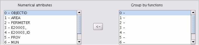
If you click on the button with the "<-" icon, a dialogue will be shown in which you can choose one of several summary functions for a selected attribute.
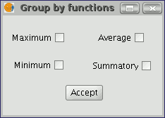
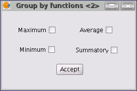
The summary functions supported are maximum, minimum, average and summatory. A field will be included in the result layer for each summary function selected for the numerical attributes you have selected a summary function for.
When you have specified the field you wish to merge and the numerical attributes you wish to obtain a summary value for in the result layer, you are ready to run the geoprocess.
Merge
Introduction
This geoprocess acts on one or several layers, generating a new layer which joins all the geometries in the “input layer”. The "result layer" of this geoprocess will keep the attributes of the "input layer" specified by the user. For the rest of the layers which have not been selected, the attributes whose name and type of data coincide with any of the attributes in the selected layer will be kept.
Example:
When a cartographic series arrives which is separated into sheets and you wish to join the content of the different sheets in one layer. This is the case of the Magna series of sheets, published by the Spanish Technological and Geomining Institute (ITGME).
Running the 'Merge' geoprocess
If you select the “Merge” geoprocess, the following dialogue appears:
The geoprocess allows any of the layers loaded in the layer tree in the gvSIG active view as an input layer. To run the process, first select the layers you wish to merge in the "Input layers" text box. Then, click on the "Select” button. A new window will open in which you can give the new layer file a name or choose a target file.
Click on the "Save" button when you have finished and gvSIG will return you to the geoprocess window. Click on the "Ok" button. This will start the geoprocess.
A new layer will be created at the end of the process which will be added to the view.
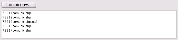
However, in the example of the sheets in a cartographic series, it would be awkward to load all the pages in the series one by one. Thus, there is an extra option to select a directory and to add all the layer files (with extensions supported by gvSIG) contained in this directory to the geoprocess input layer list. The only layer files currently supported are shp format files. If you click on the “Folder with files...” button and select a directory, a list of the layer files contained in it are shown and can be selected as part of the geoprocess input layers.
Until you select at least one layer to merge with one of the two possible lists (the layer list in the gvSIG layer tree and the layer list contained in the specified directory), no layer will be shown in the pull-down list. This list allows you to select which layer is going to define the attributes of the result layer’s attributes. When you select the layers to merge in one of the two lists, the layer whose attributes we wish the result layer to have and when you have specified the file you wish to save the result layer in, you can run the geoprocess. An initial requirement is that all the geoprocess input layers have the same type of geometries.
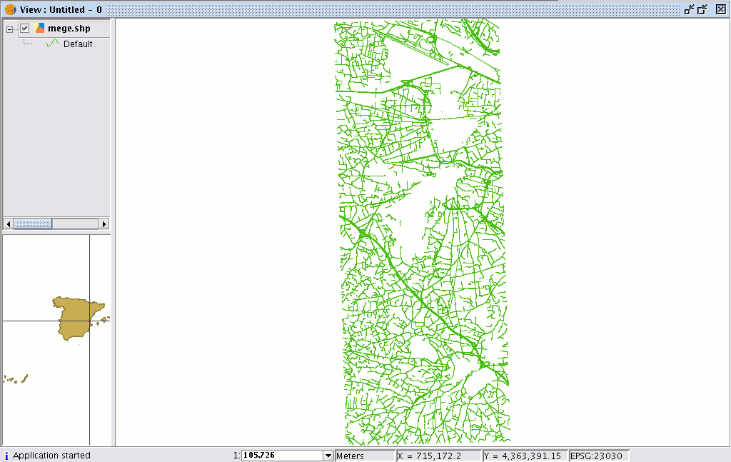
The result will be a new layer with all the input layer geometries.
Convex hull
Introduction
This geoprocess calculates the “Convex hull”, or the smallest convex polygon which surrounds all the vector elements in an “input layer”.
It only works with an “input layer” whose geometry type can be any type (point, line or polygon). There are different types of applications for this geoprocess: Determining the coverage area for a specific geographical phenomenon.
Calculating the diameter of the area covered by a series of geometries, etc.
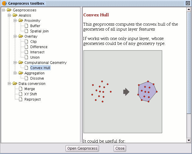
Creating a convex hull
If you select the “Convex hull” geoprocess, the following dialogue appears:
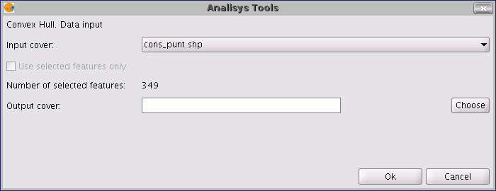
After selecting the layer whose “Convex Hull” you wish to calculate and specifying an shp result file, you can run the geoprocess and generate a new result layer.
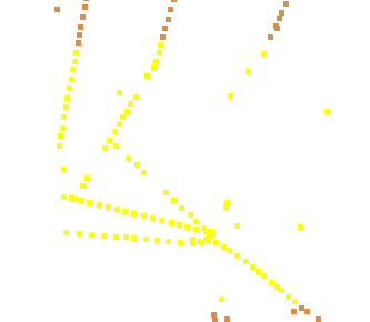
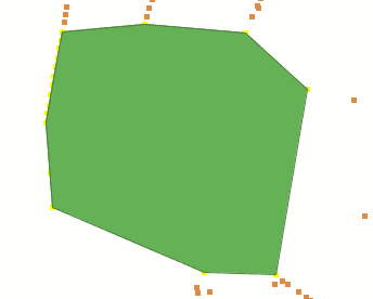
The following image shows the convex hull created which surrounds all the points in the input layer.
Difference
Introduction
The “Difference” geoprocess works with two layers, the “input layer” and the “overlay layer”. It is known as “Spatial NOT” and allows you to obtain the areas in a layer which are not present in the other layer. The geometries in both the “input layer” and the “overlay layer" must be polygons, lines or points. The alphanumerical schema of the “input layer” will remain intact in the "result layer", as in the end it gives more information about it.
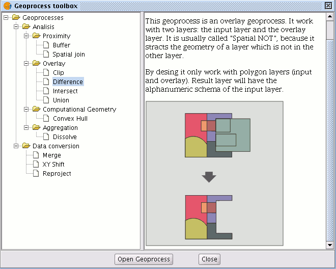
This geoprocess is very useful in numerous situations. For example, it can be used to complement the "Clip" geoprocess. If “Clip” allows you to exclude everything that does not belong to a geographical area under study, "Difference" allows you to do exactly the opposite; exclude a specific area from our working layer.
A useful example:
Transferring territorial jurisdiction between different governing bodies. Thus, if the national government transfers certain jurisdiction to a regional authority, it can decide to exclude the geographical area of the transfer in question from its data bases.
Running the 'Difference' geoprocess
Running the “Difference” geoprocessClick on the “Open Geoprocess” button to access the dialogue window which allows you to run the "Difference" geoprocess.
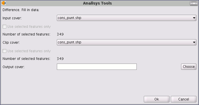
You can enable the “selected features” check boxes at this point of the geoprocess for the input layer and the overlay layer. If you click on the “Ok” button, the geoprocess will be run.
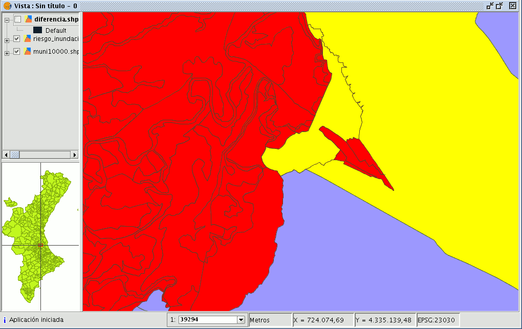
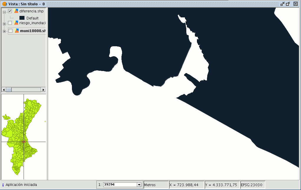
In the following image, the “Difference” geometry appears in black between a flood zone and one of the selected cities or towns. In this case, the new layer resulting from the calculation of the difference will take the schema (alphanumerical attributes) of the geoprocess input layer.
Union
Introduction
This geoprocess is similar to the “Intersection” and "Difference" geoprocesses in that it operates on two polygon, line or point layers to obtain their intersections (this is why these three geoprocesses are known as “overlay geoprocesses”).
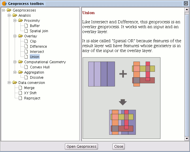
The "Union" geoprocess is known as "Spatial OR", because the result layer is made up of the geometries which appear in the two layers (intersections between the polygons, lines or points), plus the geometries which only appear in one of the two associated layers.
This means that the geoprocess carries out three analyses:
the first time it calculates the intersection of both layers, the second time it calculates differences between the first layer and the second, and the third time it calculates the differences between the second layer and the first.
This geoprocess may be of interest if you wish to generate new layers which show the occurrence of two phenomena so that the occurrence of one of the two or of both is highlighted.
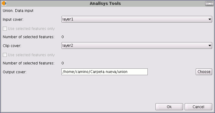
Running the "Union" geoprocess
If you select the “Union” option, the following dialogue appears:

When you have selected the input layer, the clip layer and an output layer, click on "Ok".
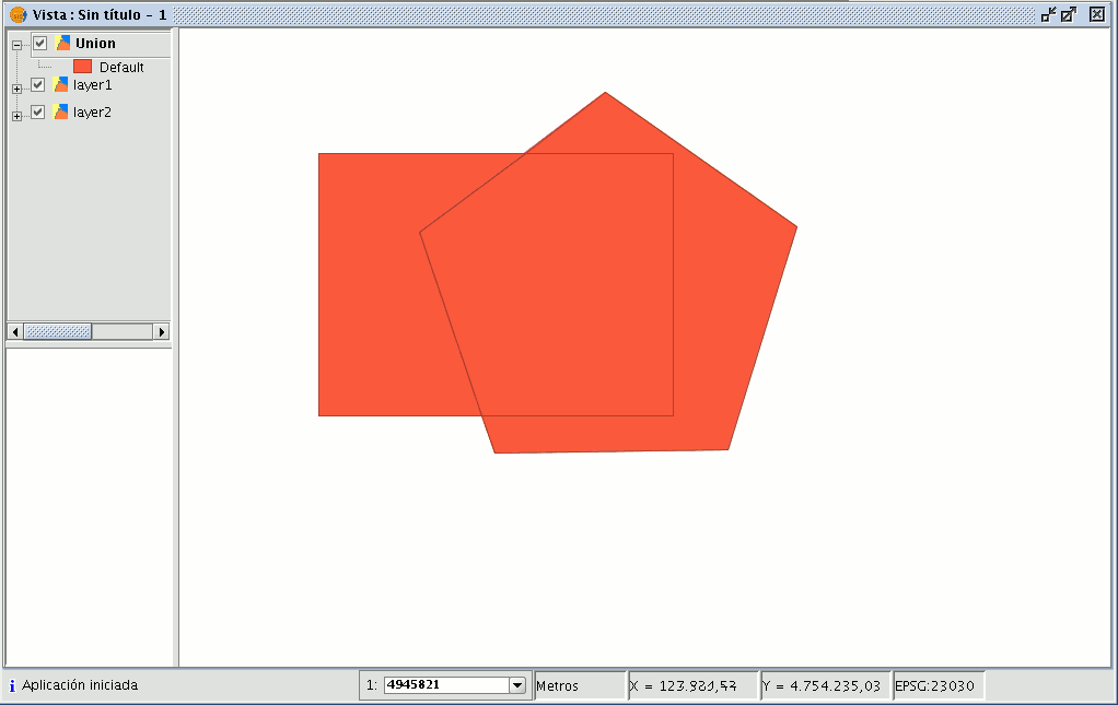
The result layer will have all the intersections and differences between the two layers. If you click on the “Information” button and then on the different polygons in the result layer, you will see that the intersections have all the attributes, whilst the differences only have the attributes of the layer that created them.
Spatial join
Introduction
This geoprocess allows you to transfer the attributes of one layer to another based on a common element. In contrast to the join sql operator in the relational data bases, in this case, the common element is not that a field of the two tables takes the same value, but that the related elements in the two layers meet some spatial criteria.
The “Spatial join” geoprocess allows you to follow two types of spatial criteria to establish the spatial link:
Nearest neighbour (1->1 relationship). This assigns the attributes of the nearest element in the related layer to an element in the source layer.
If the nearest element intersects (or in the case of polygons is “Contained in”) with the source element, the algorithm will take the first element analysed in the possible intersections.
Contained in (1->M relationship). This relates an element in the source layer with several elements in the destination layer (in particular, with those that intersect).
In this case, the source layer will not inherit the related layer’s attributes, but the operation will be very similar to the "Dissolve" geoprocess.
The user can choose one or several summary functions (average, minimum, maximum, summatory) to be applied on the numerical attributes of the related layer for the M elements related to an element in the source layer.
Running a 'Spatial Join'
When you have selected the "Spatial join" option, the following window appears:
This window is practically the same as the windows in the overlay geoprocesses (Union, Difference, Intersection) with one difference.
It allows you to choose whether you want to run a 1-1 relationship (using the nearest neighbour spatial criterion) or run a 1-N relationship (using the “Intersect” or “Contained in” spatial criterion).
The choice can be made by enabling or disabling the "Use nearest geometry" check box. If when you have selected the source layer and the layer to be related, the geoprocess is launched and you have not enabled the "Use nearest geometry" check box, a window appears in which you can select the summary functions you wish to apply for each numerical attribute of the layer to be related:
The summary functions are the same as in the “Dissolve” geoprocess:
Thus, the attributes transferred to the source layer will be the result of the summary functions selected for each numerical field. If you run the geoprocess and the “Use nearest geometry” option is enabled, this window does not appear.
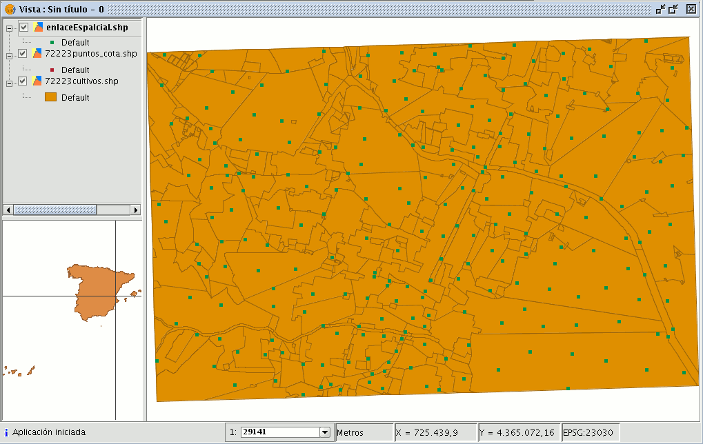
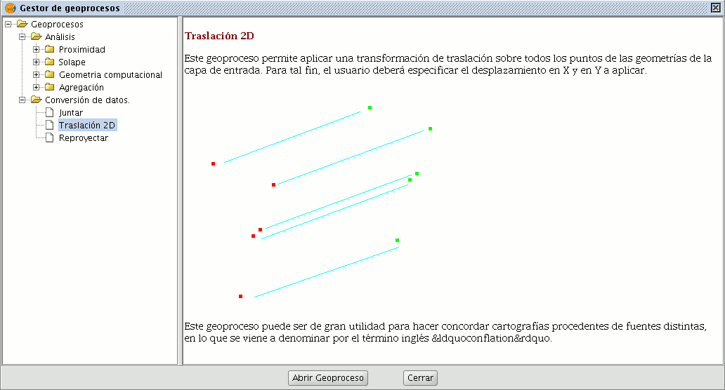
2D Translation
Introduction
This geoprocess allows a translation transformation to be applied to all the points, lines and polygons of the geometries in the input layer. The geoprocess can be applied to all types of vector layers (shp, dgn, dxf…). To do so, the movement on X and Y must be specified.
This geoprocess is extremely useful when combining cartographies which come from different sources, a process which is referred to as conflation. Bear in mind that although translations can be carried out on all types of vector layers (shp, dgn, dxf, dwg…), the resulting output layer will always be a shape file. In other words, the input layer can be a shp, dxf or dgn file, but when translation is applied to these layers, the result will be one or various different output layers which are always shape files.
When a translation is carried out in which the input layer is a vector layer which is not a shape file, the result of the translation will be three layers in SHP format (one line layer, one point layer and one polygon layer).
If, for example, the input layer to which the translation is applied contains only points and lines, the polygon .shp file will be created but it will be empty.
NB. At the end of this section there is a table giving details of the relationship between the type of input file and the resulting output layer.
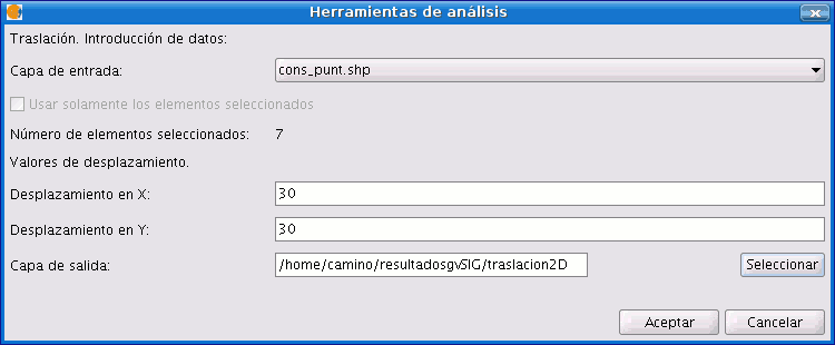
Translating a vector layer
Firstly, load a vector layer in gvSIG and then click on the geoprocessing wizard in the tool bar.

Select the option “2D Translation” from the “Data Conversion” folder. Click on the “Open Geoprocess” button and the geoprocess data input window opens. For the input layer, select the vector layer (dgn, dxf, dwg, shp…) you wish to translate and introduce the values corresponding to X and Y. Select an output layer and click on “Ok”.
The following image shows the result of applying the translation process.
Relationship between the type of layer before and after translation.
| Input cover | Output cover/s | |
|---|---|---|
| Point Shp file | Point Shp file | |
| Multipoint Shp file | Multipoint Shp file | |
| Line Shp file | Line Shp file | |
| Polygon Shp file | Polygon Shp file | |
| Dxf (points, lines, polygons) | Point Shp file Line Shp file Polygon Shp file |
|
| Dgn (points, lines, polygons) | Point Shp file Line Shp file Polygon Shp file |
|
| Dwg (points, lines, polygons) | Point Shp file Line Shp file Polygon Shp file |
|
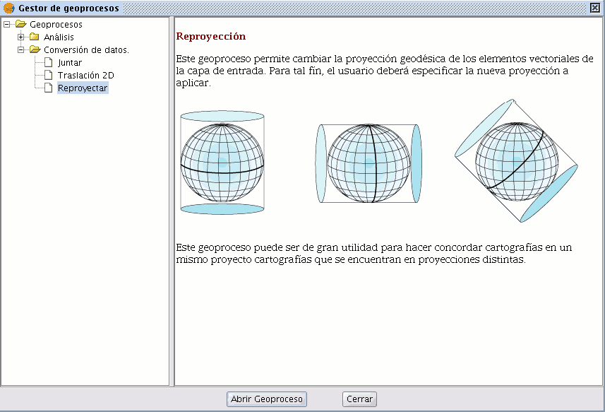
Reprojection
Introduction
This geoprocess allows you to change the geodesic projection of the vector elements in the input layer. In order to do so, the user must specify the new projection to be applied.
This process is extremely useful when standardising cartographies in the same project if these are in different projections.
Reprojection of a layer
Click on the geoprocessing wizard in the tool bar and select the “Reproject” option from the “Data conversion” folder.
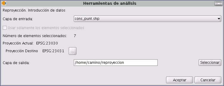
Click on “Open geoprocess”. The wizard will open to guide you through the reprojection process.
In “Input layer”, select the layer you wish to reproject from the layers loaded in the ToC.
To select the new projection for the layer, click on the button next to the destination projection and select the new reference system.
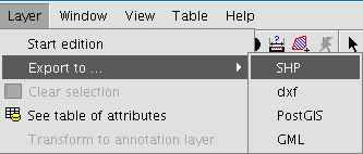
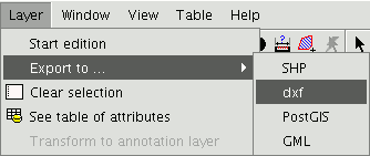
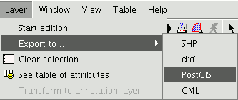
Exporting layers
Introduction
The “Export to...” tool allows you to save the elements selected in a layer in a different format. If no elements have been selected the whole layer will be exported. At the time of going to press the export formats supported by gvSIG were shape, dxf, and postgis and gml.
Exporting a shape
Select the “Layer” option from the menu bar then go to “Export to…/shp”.
If you have selected elements in the layer to be exported, gvSIG will tell you how many elements are going to be exported and will ask for confirmation before carrying out the operation.
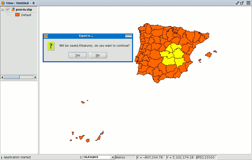
If you continue with the operation, a dialogue box will appear in which you will be asked to select the file the new shape is to be saved in.
When you have accepted, a new message will appear asking whether you wish to insert the new layer into the view.
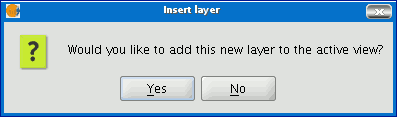
If you click on “Yes”, the layer will be added to the active view.
Exporting to dxf
Select the “Layer” option from the menu bar then go to “Export to…/dxf”.
Follow the same process used for exporting to shape.
Exporting to postgis and Oracle Spatial
Select the “Layer” option from the menu bar then go to “Export to…/postgis”.
If you have selected any elements, a window will appear telling you how many elements are going to be exported (as in exporting to shp and dxf).
If you have selected any elements, a window will appear telling you how many elements are going to be exported (as in exporting to shp and dxf).
Remember that if the table already exists in the data base, the information it contains will be deleted.
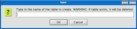
Write the name of the table and click on “Ok”. A new window appears in which you will have to input the parameters of the data base connection.
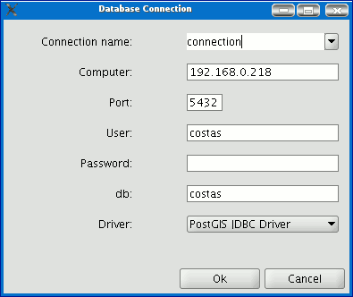
he parameters are:
Name: Name of the connection.
Computer: IP address of the computer the data base is hosted in
Port: Port on which the computer is listening to the postgreSQL service.
User: User name recognised by the administrator to make the connection
Password: User password required to validate the connection. db: The data base the new table is to be created in.
Driver: Driver required for the data base. (At the time of going to press, drivers for postGIS and mySQL were available). When you have input the connection parameters, click on “Ok”.
Exporting to gml
Select the “Layer” option from the menu bar then go to “Export to…/gml”.
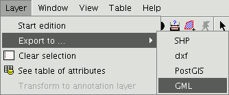
Follow the same process used for exporting to shp or dxf.
Exportar a kml
From the menu bar, select Layer > Export to... > Keyhole Markup Language (KML).
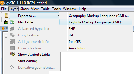
Layer menu, Export to KML
From here on the steps are exactly the same as for the Exporting to GML option.
Annotation layer
Introduction
This gvSIG tool makes advanced labelling easy.
The process creates a new layer which represents annotations.
The main features of this new layer can be summarised as follows:
- The new layer is only composed of the annotations created.
- The table associated with this new layer only contains the fields which refer to the text of the annotations (Text, Font, Colour, Height and Rotation).
- The layer created is always in .shp format, irrespective of the format of the original layer.
Creating an annotation layer
To create an annotation layer, first select the layer from the ToC (Table of Contents).
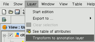
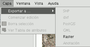
In the menu bar, select the “Layer” option, then select “Export to” and finally select the “Annotation” option.
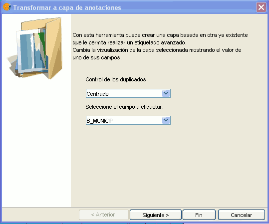
This option opens the wizard which will guide you through the steps required to create the annotation layer.
In the wizard’s first window, select the data which gvSIG requires to carry out the operation from the pull-down tab:
Duplicate control: Select either “None” or “Centred” to choose the position in which you wish the annotations to be inserted.
Centred: A label is created for each value and this will be inserted in the centre of all the labels which are the same.
None: A label is inserted for each value, even if these are repeated.
Select the field to be labelled: Choose the field which contains the text you wish the labels to show.
If you do not wish to modify the format of the annotations created by gvSIG and prefer a standard format, click on “Finish”. If you wish to customise the format, click on “Next”.
The wizard’s second window allows you to select the fields of attributes of a a table (if there are any) which contain the values which allow you to customise the labelling.
The following parameters can be customised.
Slope – the slope the annotation will have in the view.
Colour – annotation text colour.
Height – annotation text height.
Units – units in which the value assigned to the “Height” field are to be measured.
The options currently available are map units or pixels.
Font – annotation text font.
Set the values to be used for customising the required parameter (by pulling down the list).
Leave the default value in the fields you do not wish to customise.
Click on “Finish” when you have input these changes.
Editing an annotation layer
An annotation layer can be edited like any other layer. To start an editing session in gvSIG, select the layer in the Table of Contents and then select the option “Start edition”.
When you start an editing session, an option appears in the menu bar called “Modify annotation”. This will allow you to individually customise the annotation you wish to change.
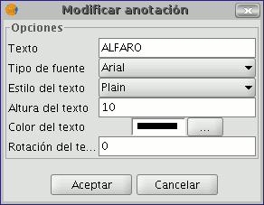
When you click on this button, the appearance of the cursor will change. You may graphically select the annotation by clicking on the point associated with the text and then access a set of properties shown in the following image.
Annotation layer properties
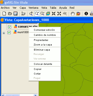
If we select the “Properties” option from the annotation layer contextual menu, the following box appears:
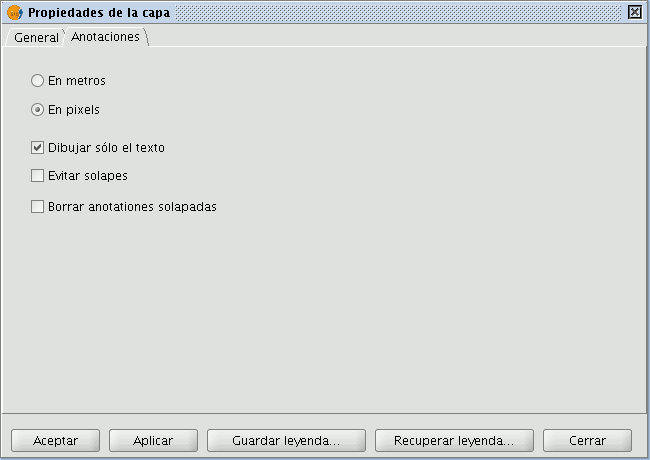
The “Layer properties” box has two tabs. The “General” tab allows you to access the general properties of the layer and the “Annotations” tab allows you to select: whether you wish the annotation text to be shown in pixels or metres in the view.
Whether you want only the text to appear (select the “Draw text only” option) or if you prefer the text to be accompanied by a location point (deselect the “Draw text only” option).
However, remember that this point is useful, for example, to move the annotation or to access the “Modify annotation” window.
If you wish to avoid overlays, activate the “Avoid overlays” option.
If you wish to eliminate overlaying annotations, activate the “Clear overlaying annotations” option.
Adding an annotation layer to the view
To add an annotation layer, click on the “Add layer” button in the tool bar

and select the “Annotation” tab.
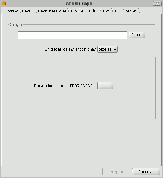
In the box you can select the annotation layer you wish to load, in addition to the units in which the annotations are displayed (pixels or metres) and the projection of the layer.
Example of how to create an annotation layer
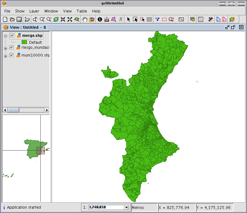
The following image shows how an annotation layer is created out of a polygon layer called “muni10000.shp” which contains all the towns in the Valencian Region.
In the first window of the wizard, insert the type of duplicate control you wish to use and select the field which contains the text to be shown.
This is the field in a layer’s table of attributes which contains the name of the town.
If you do not wish to customise the presentation, click on “Finish” and indicate where you wish the new annotation layer to be saved.
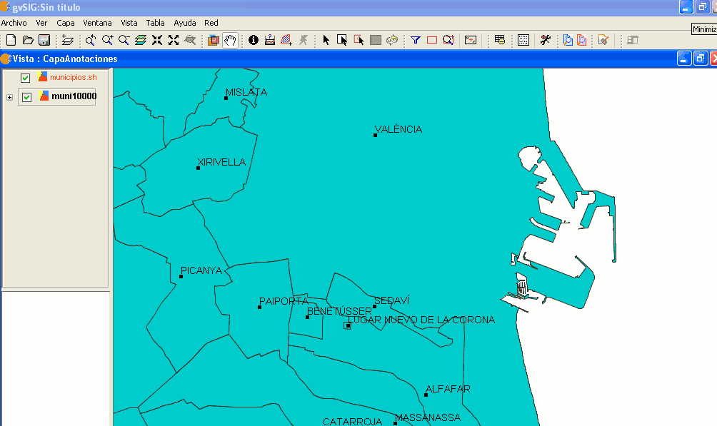
The following image shows the result (the rest of the fields in the wizard are left with their default values and this one is zoomed in) of creating the “annotation layer”.
The annotation layer which has been created is the one in red called “Towns” in the Table of Contents.
Export to a raster layer
This tool allows you to extract portions of a raster layer using a selection in the view or by inputting the coordinates that define the portion to be extracted.
It allows the user to change the spatial resolution of the clipping or of the whole image, choose the bands to be extracted or generate a new raster layer for each of the original bands.
To access this option, go to the ToC and select the raster layer you wish to select a portion of.
Then go to the Layer/Export to menu and select the “Raster” option.
The following window appears:
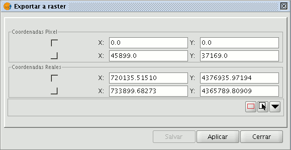
Image clipping
There are two ways of selecting an area to be clipped from the original raster layer:
You can use the text boxes in the window to input the data which correspond to:
- Real coordinates: If the source image is georeferenced.
- Pixel coordinates: If the source image is not georeferenced.
You can also make your selection directly from the view by clipping the whole image or selecting a part of it.
This button allows you to obtain a clipping from the whole image.
This button allows you to obtain a clipping from a selected area in the view. Place the cursor over the image, then click and drag. Check that the text boxes are automatically completed.
If you wish to save the raster layer clipping you have created, click on “Save” and select the location you wish to save this file in. The image will be saved in TIF format.

Changing spatial resolution
The controls that allow you to specify the clipping’s (or whole image) spatial resolution are located in the Clip table, with the additional options panel pulled down (to pull this panel down click on the button). You can define the resolution by specifying the Cell size or the Width and Height of the raster layer to be generated in pixels as well as choosing the interpolation method using the resolution change. At the moment, only the “Nearest neighbour” option is operational.

Band selection
The original raster layer’s band list appears at the bottom of the Clip table. You can use this list to choose the bands the output raster layer will have if you enable or disable the check boxes in the Bands column. If you check the Create one layer per band option, a new layer will be generated for each of the bands checked in the list. The new layers will be added to the ToC.
Saving and Adding a raster layer clipping to the current view.
When you have established all the parameters which define the raster layer clipping you have made, click on “Save”. This opens a dialogue box which allows you to search for a directory to save the clipping in. If you wish to add the layer to the view, go to the “Add layer” button in the tool bar once you have saved the clipping.
Example of a raster layer clipping
This example shows how a clipping is taken from an orthophoto.
First, select the area by defining a rectangle in the gvSIG view.
When you have finished, the coordinates will automatically be input into the text boxes based on the selection. You can fine tune these selected values from the view by inputting the new value directly into the text boxes containing the data.
Then pull down the box. As the resulting image is to be resampled, not as much resolution is required. Therefore, go to the “Spatial resolution” section and select “Width x Height”. This enables the text boxes so that you can input the output raster layer resolution.
When one value is input the other one is automatically completed when you press Enter or when you exit the field, as the proportions between the width and height must be maintained.
The cell size for the chosen output resolution is also calculated. If “Cell size” had been chosen, you would have had to specify the size in metres for each pixel and thus the width and height for the chosen cell size would have been calculated.
You now need to select the bands you want the output layer to have. In this case, select them all as this is a three-band orthophoto and we want to include them all.
Finally, for our example, the “Create a layer per band” option needs to be enabled to do just this.
Each new layer will have the same data type as the original image. If you click on “Save” a dialogue box opens to indicate the directory and image name.
To retrieve the layers you have created, go to the Add layer” button and then to the directory they were saved in.
Crear shape de geometrías derivadas
"New layer with derived geometries" tool.
This tool allows users to generate geometries derived from points or lines in a vector layer, and to store them as a new shape layer.
| Icon | Description |
|---|---|
 |
Derived geometries tool enabled if the TOC contains at least one visible point or line vector layer that is not in edit mode. |
 |
Derived geometries tool disabled if the TOC does not contain any visible point or line vector layers that are not in edit mode. |
The tool can be accessed from:
Via the menu: Layer / Derivative geometries
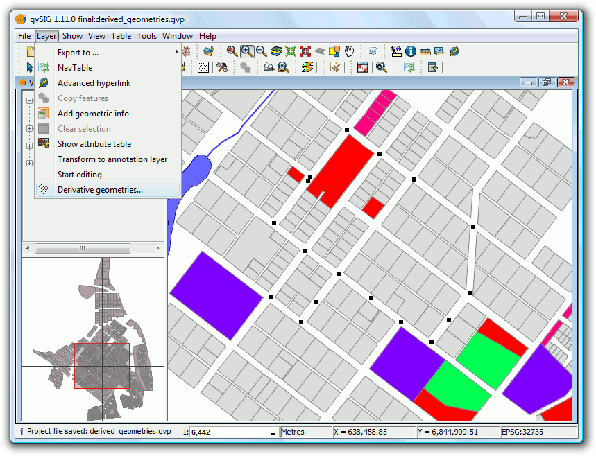
Menu path to the tool
Layer selection dialog and process
Upon choosing the tool a dialog for selecting layers is displayed:
Selecting layers and process
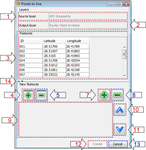
- Source Layer: drop-down list of point or line vector layers in the current View that are not in edit mode. Select a layer to be the source layer.
- Name of the output layer: layer name that will appear in the TOC.
- Path of the output layer: full path for creating the new shapefile.
- Type of output layer: geometry type of the new layer. This depends on the type of process chosen (See options below).
- Type of process: select the type of geometry generation process. This depends on the geometry of the source layer. This process is applied to the source and destination layer pair until the tool is closed.
- Cancel: Close the tool.
- OK: Opens a control panel and displays data for the selected source layer. This control panel will be associated with source and output layers until it is cancelled.
| Source layer geometry type | Type of process | Target layer geometry type |
|---|---|---|
| Points | Points to line | Lines |
| Points | Points to polygon | Polygons |
| Lines | Close polylines | Polygons |
Process Control Panel
The control panel is associated with the layer and is shown every time the layer is activated in the TOC, as long as the layer is visible and not in edit mode.
The dialog has a semi-modal behavior in order to allow the user to continue working with gvSIG by using the minimize, maximize, resize and hide buttons (use the X, not the Cancel button, to hide the dialog).
Process control panel
- Name of the source layer: Layer from the TOC that contains the source geometries.
- Name of the output layer: Name of the new derived geometry layer that will appear in the TOC.
- Table of features: Table showing the attributes of all the source layer's features. Source layer geometries selected in the View will also be selected in this table.
- Add all: Adds all the features of the source layer to the table of selected features.
- Remove all: Removes all features from the table of selected features.
- Enable snapping tool: Enables snapping tool on the source layer, without putting it into edit mode (only available in the Castilla y León extension for gvSIG 1.1.2).
- Add selected features: Adds only the selected features to the table.
- Remove selected features: Removes only the selected features from the table.
- Table of selected features: Table showing the attributes of all the features selected from the source layer. It has 2 extra columns:
- Order: Order to be used when generating the new geometry from the selected features in a point source layer, or when closing polylines in the case of a line source layer. The order can be changed with buttons 10 and 11.
- ID: Fixed ID number of the geometry in the vector layer.
- Move up: Moves the selected geometries up one position.
- Move down: Moves the selected geometries down one position.
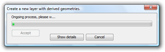
- Create: Start the process of generating the derived geometries. If it doesn't already exist, a new layer is created, and the new geometries are added to this layer. The process is done in a thread, the progress of which is indicated by a progress bar.
Progress bar
The results of the completed process can be viewed by clicking on the "View Details" button. There are three types of data that are of interest here:
- Number of geometries to create: depends on the geometry selected:
- If they are of type point: one line or polygon is created.
- If they are of type line: one polygon is created for each line.
- Number of geometries that could not be created: the subprocess failed, for example because a polygon couldn't be derived from simple lines that consist of only two points.
- Number of geometries created successfully: the new geometries created.
 This information is recorded in the gvSIG log.
The control panel is hidden during the process but becomes visible again when the progress dialog is closed.
- Cancel: Closes the control panel and de-registers the associated tools, thereby terminating the tool for the specified source layer.
- Expand / Collapse: Changes the position of the splitter, so as to display only the table of features, only the table of selected features and associated management controls, or both halves of the control panel interface.
Control Panel Behaviour
The control panel is linked to the source layer from the time it is created until it is cancelled by clicking the cancel button.
| Action | GUI Element | Description |
|---|---|---|
| Maximize |  |
Resizes the dialog so that it fills all available space. |
| Minimize |  |
Minimizes the control panel to a restore button. |
| Collapse |  |
Control panel is hidden but remains linked to both the source and output layers. Further operations between these layers can be performed once the panel is restored. |
| Resize | The size of the control panel can be increased or reduced by selecting and dragging the edge of the panel. | |
| Expand / Collapse splitter interface |  |
These controls are used to display only the table of source layer features, or only the table of selected features and associated management controls, or both halves of the control panel interface. |
| Cancel |  |
Closes the tool so that is no longer available for operations between the source and output layers. |
When the control panel is hidden it can be restored it by clicking on the source layer in the TOC.
If the View is closed when control panels are visible, the panels will be hidden and then restored when the View is reopened.
 Geometries derived from points do not retain any attribute values but do maintain the columns. Those derived from lines, keep all attributes.
Removing the new layer associated with control panel will result in the tool being ended and a warning being displayed to the user.
Examples
This example will show how to generate a line layer showing the path followed from home to work, and back again. The example uses the following four shape layers:
- Land-use: layer showing parcel boundaries of the town.
- Rivers: layer showing rivers in the town.
- Lakes: layer showing lakes in the town.
- GPS Waypoints: shape layer containing points recorded by a GPS on the drive to and from work. This layer will be used as the source layer in the example.
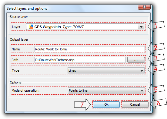
Once all four layers have been loaded the "Derived Geometries" tool can be selected and the following values entered:
- Source layer:
- Layer: GPS Waypoints
- Output Layer:
- Name: Route: Work to Home
- Path: .../RouteWorkToHome.shp
- Type: Lines
- Options:
- Mode of operation: points to line
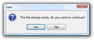
When "OK" is clicked the new process control panel appears. If a file with the same name as the new output layer already exists then the user is asked whether to continue or not. If yes, then the file will be overwritten.
Warning of an existing layer
Minimizing the control panel will reveal the View:
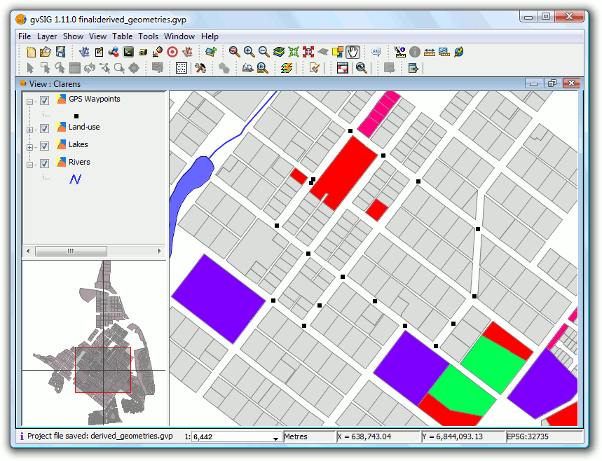
View showing the layers
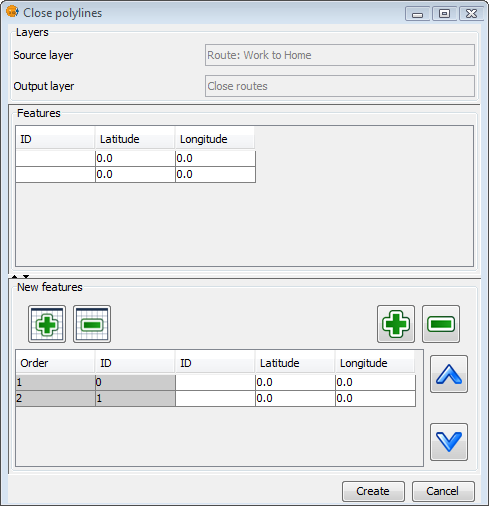
The geometries can be selected from the top table in the control panel.
We select the first seven geometry points (1st route: work to home).
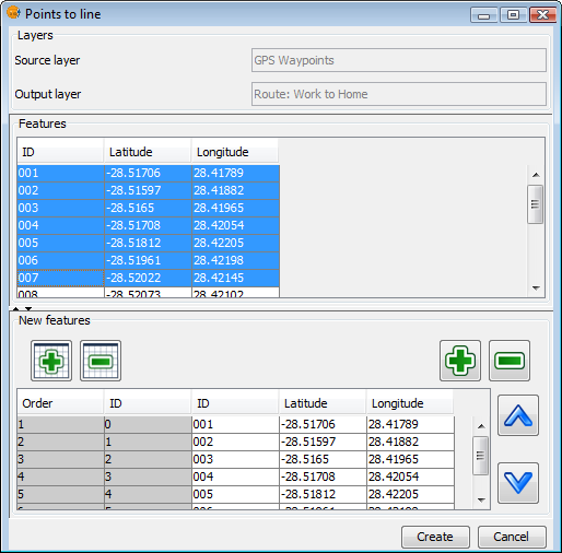
Selected geometries
Click "Create" to generate the first path:

Resulting route generated by the "Points to line" process
Modify the symbology so that the route stands out as a thick line.
To generate the route back, activate the control panel and select the remaining points from the source layer so that the line can be generated:
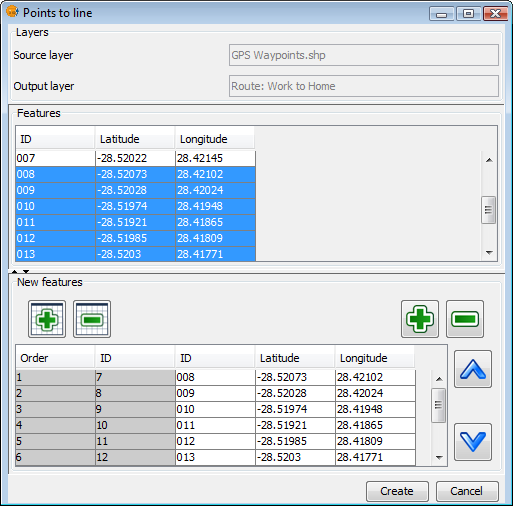
Selected geometries

Resulting new route
Finally suppose we are interested in the polygon formed by the closure of the routes.
Cancel the tool and then reopen it but this time use the new layer as the source:
- Source layer:
- Layer: Path: GPS Waypoints
- Output Layer:
- Name: Close routes
- Path: .../CloseRoutes.shp
- Type: Polylines
- Options:
- Mode of operation: close polylines
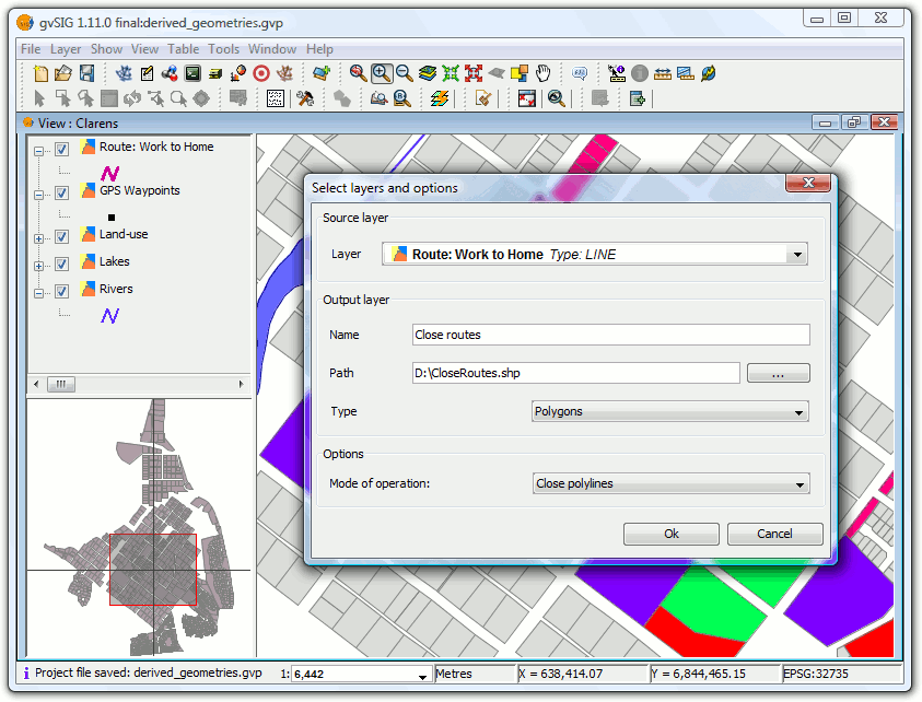
Process "close polylines"
Select all the geometries (the two polylines) and generate the polygons.
Selected geometries
Since the layer "Route: Work to Home" does not contain data due to the points to line process, we assign a distinguishing identifier to each by editing the layer.
Now apply some changes to the symbolology:
- Layer "Close routes": select a unique values symbology to distinguish the two polygons, and choose fill patterns that allow the lower layers to be seen.
- Layer "GPS Waypoints": Use a symbol of a car for the points and place the layer above the other layers.
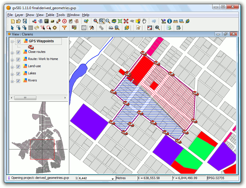
Results of the polygons generated by the "Close polylines" process
Raster
Layer functionalities
Filters
Description
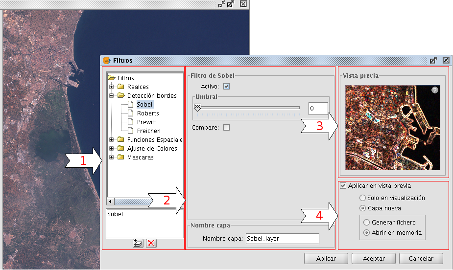
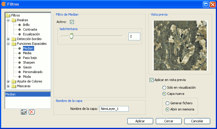
Filtering is a process by which we can enhance images. gvSIG can filter images through a variety of filtering methods. In the upper left part of the Filter dialog, the filters are grouped by type (1). By double-clicking one of the filters or by clicking on the "Add Filter" button on the bottom left, the filter will be added to the list of filters in the lower left part of the Filter dialog. All filters in the filter list will be applied in the preview. If you want to remove a filter from the list, you can either double-click on the filter or click on the "Delete filter" button. The filters in the list will be applied to the image in the order that they appear. Keep in mind that the order in which the filters are applied will affect the result, and changing the order of the filters may change the output.
In the middle of the dialog window are the controls of the selected filter (2). When changing the controls of one of the filters from the filter list, the results will be directly shown in the preview window. Below the middle part of the dialog you can change the name of the output layer that will be generated when clicking "Apply" or "Close".
On the right side of the dialog you can preview the outcome of the filters (3). (See documentation on "Preview tool"). In the lower right part you can select whether you want to display the filters over the selected layer or save the filtered image as a new layer (4).
The button "Apply" will apply the changes according to the entered parameters, keeping the Filter dialog open. The "Close" button will apply the changes and close the Filter dialog. The "Cancel" button will close the Filter dialog without applying any filters.
All filters in the filter list can be activated or de-activated through the "Active" checkbox. This checkbox is usually located in the upper part of the filter control panel.
Configuration panel for the image filters
Generate a new layer or apply to current layer
The number of applied filters will affect the time that it will take to draw the layer. If you choose to apply the filters to the current layer, the drawing and re-drawing of the layer may slow down while the filters are applied. If the filter results are saved as a new layer, the filtering process has to be done only once so that the next time the layer is drawn, it will not be slowed down by the filtering. Therefore, it is generally recommended to save the output to a new layer if possible. There are cases though in which it is not recommended to generate a new layer. For example, if you have a large orthophoto and you only want to change the brightness a little, it could take more time to save the output as a new layer. If the brightness filter is applied over the current view, the area on which the filter is applied is much smaller which makes the drawing faster. It is up to the user to decide whether it is better to create a new layer or display the filters on the view of the current layer.
Enhancements
The brightness filter changes the brightness value of the layer. You can increase or decrease the brightness by moving the position of the sliding bar or by entering the value directly in the text box and press enter.
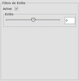
Brightness filter
The contrast filter changes the contrast value of the layer. You can increase or decrease the contrast by moving the position of the sliding bar or by entering the value directly in the text box and press enter.
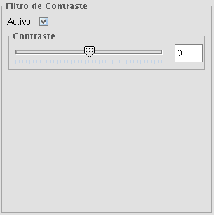
Contrast filter
Spatial filters
With this type of filter, graphical transformations like smoothing, edge detection, sharpening etc. are applied to the image.
The following filter types can be applied:
MEDIAN FILTER
The median filter applies a kernel of a certain size, which is determined by the user through the sliding bar labeled Window side.
The median filter is normally used to smoothen and to reduce noise in an image, by moving a kernel of N x N number of pixels over the image and evaluating each central pixel, replacing its value with the median of its neighboring pixels. Compared to the Mean filter, the advantage of the Median filter is that the final pixel value is a value that actually occurs in the image and not an average.
Median filter
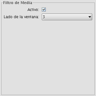
MEAN FILTER
The mean filter applies a kernel of a certain size, which is determined by the user through the sliding bar labeled Window side.
The filter replaces the value of the central pixel with the mean value of the surrounding pixels. Each value of the kernel would be one and the divider would be the total number of elements in the kernel (i.e. a kernel of 3 x 3 would replace the value of the central pixel by the average value of the nine pixels covered by the kernel).
Mean filter
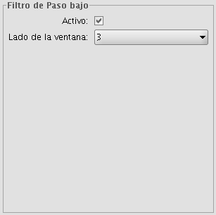
LOW PASS FILTER (smoothing filter)
The low pass filter applies a kernel of a certain size, which is determined by the user through the sliding bar labeled Window side.
Using a low pass filter tends to retain the low frequency information within an image while reducing the high frequency information.
Low pass filter
SHARPENING FILTER
By moving the slider to change the sharpness (values from 1-100), the contrast of an image can be changed. The results can be evaluated in the preview window. With a higher contrast, details in the image can be accentuated but the noise will also increase.
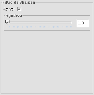
Sharpening filter
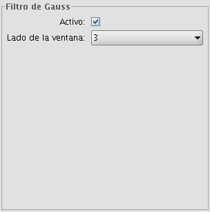
GAUSS FILTER
The Gauss filter applies a kernel of a certain size, which is determined by the user through the sliding bar labeled Window side.
The maximum value appears in the central pixel and gradually decreases for pixels that are further away from the central pixel.
Gauss filter
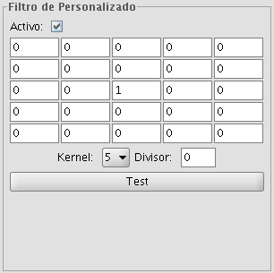
CUSTOM FILTER
This is a kernel of 5 x 5 or 3 x 3, for which the values can be introduced by the user. After multiplying the pixel values with the kernel values, the result will be divided by the number specified in the Divisor textbox.
Custom filter
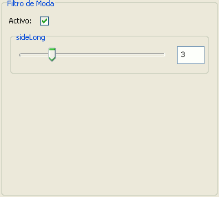
MODE FILTER
The mode filter applies a kernel of a certain size, which is determined by the user through the sliding bar labeled Window side.
This filter takes the value that occurs most in the surrounding pixels and assigns it to the central pixel.
Moda filter
Colour adjustment
Adjustment of RGB values
It is possible to change the balance between Red, Green and Blue in an image if needed. To do this, move the sliding bar to increase or decrease the values or enter the value directly in the text box next to the sliding bar. Ticking the "Brightness" check box ensures that the brightness level of the pixels will be maintained while the RGB values are changed.
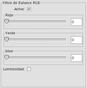
RGB balance filter
Adjustment of CMY values
It is possible to change the balance of Cyan, Magenta and Yellow in an image if needed. To do this, move the sliding bar to increase or decrease the values or enter the value directly in the text box next to the sliding bar. Ticking the "Brightness" check box ensures that the brightness level of the pixels will be maintained while the CMY values are changed.
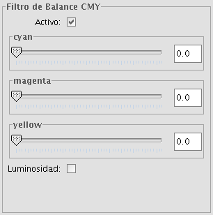
CMY balance filter
Adjustment of HBS values
It is possible to change the balance of Hue, Brightness and Saturation in an image if needed. To do this, move the sliding bar to increase or decrease the values or enter the value directly in the text box next to the sliding bar.
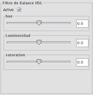
HBS balance filter
Edge detection
These filters attempt, through the use of kernels, to detect edges in the image and change the image so that these edges are enhanced, while the rest of the image is grayed out.
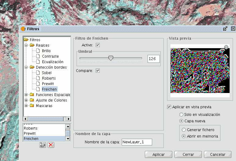
Filter dialog. Edge detection
There are four edge detection filters, all with the same interface and options, in which the user chooses a threshold in the range 0-255, and the possibility compare the results by ticking the compare check box:
Sobel filter example
SOBEL
The Sobel filter detects the horizontal and vertical edges separately on a grayscale image. Colour images are converted to RGB gradations. The result is a transparent image with black lines and some remains of colour.
ROBERTS
The Roberts filter is suitable for detecting diagonal edges. It offers good performance in terms of location. The major drawback of this filter is its extreme sensitivity to noise and therefore has poor detection qualities.
PREWITT
The Prewit filter detects edges in all directions as it consists of 8 kernels that are applied over the image pixel by pixel.
FREI-CHEN
The Frei-Chen filter processes the neighbouring pixels as a function of their distance from the pixel that is being evaluated. The result is that edges in all directions are detected.
Masks
Transparent area
With this functionality it is possible to set the transparency level of a Region of Interest (ROI). The region of interest must have been defined previously. If the layer does not have a region of interest, the following message will appear: "A Region of Interest (ROI) must be defined for this layer to apply this filter. Please go to the dialog Area of Interest and select at least one ROI." If there are already one or more ROI associated with the layer, the message will not appear. Instead, a list of ROI will be shown, from which you can select one or more by ticking the corresponding check box. Then, adjust the level of transparency with the slide bar or by entering the value directly in the text box next to the slider. Ticking the check box labeled as "Inverse" will result in the opposite effect; all of the image except for the ROI will be set to the specified transparency level.
Transparent area filter
Mask
With this functionality it is possible to cut out a Region of Interest (ROI) that has been previously defined for the layer by assigning a fixed user-specified value to the rest of the image outside the ROI. If the layer does not have a region of interest, the following message will appear: "A Region of Interest (ROI) must be defined for this layer to apply this filter. Please go to the dialog Area of Interest and select at least one ROI." If there are already one or more ROI associated with the layer, the message will not appear. Instead, a list of ROI will be shown, from which you can select one or more by ticking the corresponding check box. Then, select the value to be assigned to the pixels outside the ROI by typing a number in the "value" text box. The default value is -99,999. Ticking the check box labeled as "Inverse" will result in the opposite effect; the ROI will be assigned the specified value while the rest of the image values are maintained.
Mask filter
Histogram
Description
To launch the histogram dialog window, use the drop-down toolbar selecting the "Raster Layer" button on the left and "Histogram" in the drop-down button on the right. Make sure that the text box that displays the current layer is set to the name of the raster layer for which you want to see the histogram.

Histogram icon
The Histogram dialog shows a histogram of the statistical distribution of pixel values in the current view. This information is often useful when you are trying to color balance an image. In the middle of the dialog you will see the graph on which you can right-click to show a context menu with general options for this kind of graphics.
Histogram dialog window
In the upper part of the dialog (1) are the controls to configure the histogram:
1. Type of histogram
There are three types: "Normal", "Accumulated" and "Logarithmic".
- Normal: This is the normal histogram in which for every pixel value on the X axis the number of pixels is shown on the Y axis.
- Accumulated: Shows the accumulated number of pixels for every pixel value. The graph is therefore ascending.
- Logarithmic: Displays the histogram on a logarithmic Y axis, which may be useful for images that contain substantial areas of a constant value.
2. Data source
With this option you can select the data source for the histogram:
Current view (R,G,B):
With this option, the pixel values that are displayed in the current view of gvSIG will be used for the histogram. Therefore, the band selector shows only the R, G, and B values which are the visual bands. Every band will appear in its corresponding colour in the graph (red for R, green for G and blue for B). This is the default option when the histogram dialog is opened.
Complete histogram:
With this option, the histogram for the whole raster layer is calculated. Because of the amount of time that it would take to calculate the histogram for large images, the histogram is only calculated once and saved with a .rmf extension in the directory in which the image is stored. After the first time, the histogram for the same layer can be displayed much faster. (Keep in mind that if you delete the .rmf file that is stored with the image, you will lose its histogram information.)
3. Band selection
Apart from identifying to which band each histogram corresponds through its colour (in case of the current view Data Source) you can also identify the band by hovering the mouse over a point in the graph. The tooltip displays the band name and the value of the point.
Zoom operations
We can zoom in and out of the graph using the mouse.
- To zoom in on a part of the graph, draw a rectangle over it by pressing and dragging the mouse.
- To return to the original graph, click on the left mouse button on any point in the graph and drag to the left, then release the mouse button.
You can also zoom in and out using the context menu.
Context menu
When you right-click on any part of the graph, the context menu is shown with the following options:
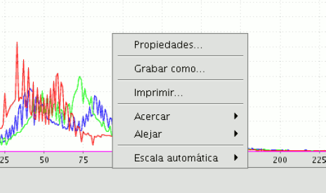
Histogram options. Context menu
- Properties: This will open the properties dialog of the graph, where you can configure characteristics such as the background colour, title, font etc.
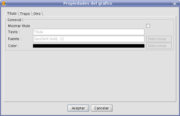
Histogram properties
- Save As: to save the graph as an image.
- Print: this opens the printer dialog from where you can print the graph.
- Zoom In: to zoom in on one or both of the axes.
- Zoom Out: to zoom out on one or both of the axes
- Auto Range: to adjust the zoom automatically to the window size, for one axis or for both.
5. Statistics (4)
The controls that appear under the graph allow the user to restrict the range of values (X axis of the histogram) on which the histogram is based. The default setting is the complete range so that, for example in a Byte data type image, the statistics are calculated for all the pixel values from 0 to 255. You can enter the values directly in the text boxes or use the + and – controls next to the text boxes. You can also slide the triangles over the sliding bar to select the range of values.

Sliding bar with pixel ranges
In this table, the statistics that correspond to the selected range of pixel values are shown in the text boxes. Each row of the table corresponds to one raster band as displayed in the histogram. The columns that are shown are:
- Minimum pixel value for the selected interval.
- Maximum pixel value for the selected interval.
- The mean (average) of all the pixel values for the selected interval in the histogram.
- Median pixel value for this interval.
- The number of pixels included in the selected interval.
6. Export the table (3)
You can export the table through the option "Save as DBF". The data contained in this table are the values of the current histogram. After creating the DBF table, it can be used as any other table in gvSIG.
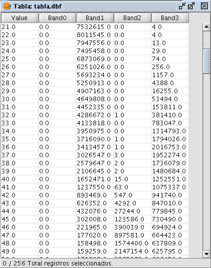
Resulting DBF table
Preferences
The Raster section of the Preferences dialog contains the option "Number of classes" where you can set the number of intervals in which the histogram is divided when the data type of the image is not Byte. For Byte images, this value is 256. In the preferences dialog, the default value of this option is 64 but you can choose any of the options (32, 64, 128, and 256). The intervals are the parts in which the range of values is divided. For example, if we have a DTM with values between 0 and 1 and there are 64 intervals, each interval will have a range of 1/64.
The number of classes does not only refer to histograms but also to other functionalities that require a division in intervals of value ranges.
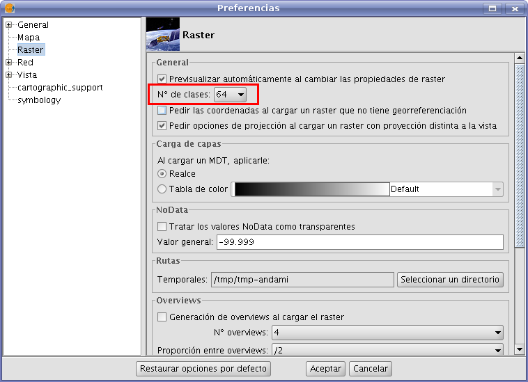
Raster Preferences
Radiometric enhancement
The maps that are obtained through digital processing of satellite imagery are useful not only for thematic mapping, but also as a backdrop on which map features can be overlaid. If the visible bands are displayed in a colour composition through the colouring of each band with the corresponding colour gun, it is important that the bands are sufficiently enhanced so that the colours appear more natural. The final display colour depends not only on the direct result of the chosen colour composition but also on the radiometric post-processing. The satellite image map will be more useful as backdrop if the bands are enhanced and displayed in colours that match the natural colours as the human eye perceives them. gvSIG provides the enhancement tools to adjust the colours for each band.
In the following sections the different parts of the dialog are described:
Histograms
The central part shows two graphs (1). The graph on the left is the histogram of the input image. The graph on the right shows the histogram of the output image. The graphs that are presented with a yellow line can be modified with the mouse. When you change the input histogram, the output histogram will be changed accordingly and you can preview the result.
In the upper corners of the input histogram are the maximum and minimum values of the raster displayed. In the lower corners, the maximum and minimum values that are being included in the enhancement are displayed. The percentage of values that are being left out of the histogram appears in parentheses. These values can be modified by grabbing and dragging the dotted vertical lines on the side of the graph. Dragging the left line will modify the minimum value, while dragging the right line will modify the maximum value. (This way, by leaving out the values that are not used in the input image, you can stretch the output values over the whole range of available values, so that the visual quality is improved.)
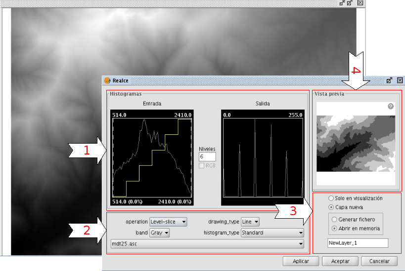
Radiometric Enhancement dialog
Controls
In the lower part of the dialog (2) you will find some controls with the following options:
Type of function:
The enhancements will replace each input value with an output value. This process is done by creating a look-up table which provides the correspondence between a range of input data and a range of output data. To apply this correspondence, a fuction is used. The used function and its parameters are chosen by the user.
Linear enhancement
- Linear: Linear enhancements apply the correspondence between the input data and output data in a linear way. In the simplest case, a straight line will correlate each value in the input interval with the corresponding value in the output interval in a complete equidistant way. For example, if you have an output range between 0 and 255 and the input values are between 0 and 1, the input value 0.5 would result in an output value of 127.5. This is the default algorithm when you first open the radiometric enhancement dialog. Variations of this algorithm can be achieved by introducing break points in the yellow line, by clicking on the line at the point where you want to break it. You can remove break points by right-clicking on them. Existing break points can be moved by dragging them. The effect is that the linear filter is divided in parts with different inclination, so that different parts will follow a different linear function as defined by the inclination of the corresponding line part.
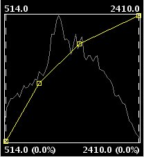
Linear radiometric enhancement
- Level slice (piecewise linear): This is a type of linear enhancement. It divides the function stepwise in equidistant parts. The effect is that the input values between two points on the same horizontal level will be assigned the same output values, so that the resulting image will have colour intervals without transitions. (This may be useful to highlight a specific range of gray levels in an image, for example to enhance certain features.) You can modify the number of intervals by changing the value in the text box labeled "Levels". The default value is 6 levels.
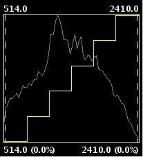
Piecewise linear enhancement
Non-linear enhancement
The non-linear enhancements have the same approach as the linear enhancements in the sense that each input value is replaced by an output value. The difference lays in the function that is assigned to produce the output values, which is non-linear. The available non-linear functions are logarithmic, exponential and square root. With each function you can modify the curve to smooth or accentuate the enhancement result.
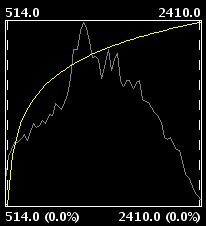
Exponential radiometric enhancement
Band
With this option you can specify the raster band to which the enhancements are applied. For a correct balance of the image, it is recommended to enhance each band separately.
Drawing type
With the option drawing type, different types of histograms can be chosen. Filled will draw a filled histogram while Line will only show the contours of the histogram. The colour of the line or fill pattern depends on the selected band. The bands Red, Green, Blue and Gray are displayed in red, green, blue and gray respectively.
Type of histogram
- Standard: Standard display of the histogram. For each possible value on the X axis, the number of pixels that are assigned this value in the output image are shown on the Y axis.
- Cumulative: For each possible pixel value on the X axis, the number of pixels that are assigned this value in the output image are shown on the Y axis. Furthermore, the number of pixels with the same or lower value are added to the result.
- Logarithmic: This shows the logarithmic value of the histogram in each position, resulting in a more balanced histogram without dominating peak values.
- Cumulative Logarithmic: This shows a cumulative histogram in logarithmic values.
RGB Check box
When check box labelled as RGB is ticked, it is assumed that the image is displayed as RGB with Byte data type and values between 0 and 255. If the checkbox is not ticked, it is assumed that the range of values are Byte data type values between -127 and 128, which will produce significant differences in the display and in the minimum and maximum values that are shown in the bottom of the input graph.
Display enhancement results
In the lower right part of the dialog (3), you can indicate how you want to see the enhancement results; in the current view or saved as a new layer.
Preview
The preview window (4) shows the real-time results of each enhancement that is applied to the image.
Save View as image
The tool for exporting the view as an image can be accessed from the drop-down toolbar by selecting "Export to raster" on the left button and "Save view to georeferenced raster" on the right button. Make sure that the name of the raster layer that you want to export is set as the current layer in the text box.

Export to raster. Save view to georeferenced raster
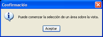
A message will appear to inform that you can use the selection tool to set the area in the view to export.
You can begin to select a area on the view
Now, you can select two points in the view to define the rectangle of the area to be exported, by clicking the first point and dragging the mouse towards the second point, then release.
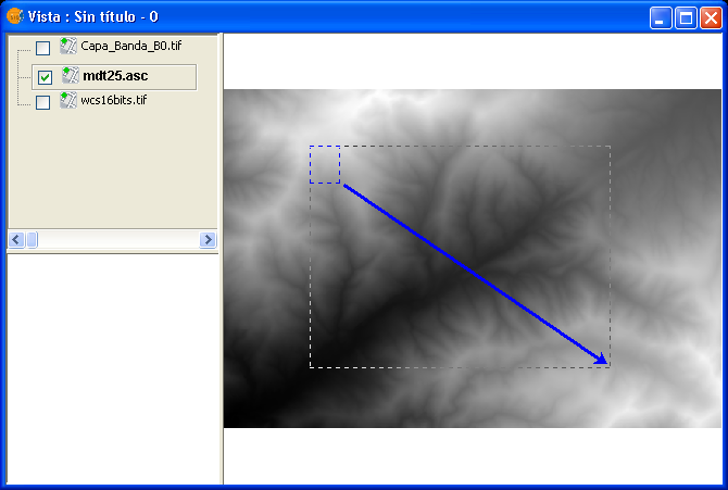
Selection of a rectangle to define the output image
Then, the Save view to georeferenced raster dialog will appear. If the selected area is too small, the dialog will not appear and a bigger rectangle must be selected.
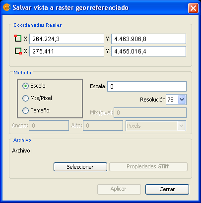
Save view to georeferenced raster dialog
The upper part of the Save view to georeferenced raster dialog shows the coordinates of the two points that define the selected area in the view. You can edit the coordinates to change the selected area.
In the option box in the central part of the dialog you can choose from three selection methods:
- Scale. Selecting this option will enable the Scale textbox and the pull-down box "Spatial resolution" which refers to the resolution in points per pixel (ppp) of the exported image. When entering a value in the Scale textbox and clicking enter, the values "Mts/pixel" and the size (Width and Height) will be recalculated for the output image.
- Mts/pixel (Meters per pixel): When selecting this option, the "Mts/Pixel" textbox is enabled. When you enter a value in the Mts/Pixel textbox and press enter, the values for "Scale" and size ("Width" and "Height") will be recalculated automatically for the output image.
- Size: When selecting this option, the text boxes to enter the "Width" and "Height" will be enabled. When you enter one of these values, the other will be calculated automatically to preserve the right proportions of the image. The other data ("Mtx/Pixel" and "Scale") will also be recalculated automatically. By default, the Width and Height values are displayed in Pixels, but you can select the units (Pixels, Cms, Mms, Mts, or Inches) in which you want to see these values.
NOTE: To save time and memory the maximum size of output images is limited to 20000 x 20000 pixels. If the intended output image is larger and you click on "Apply", gvSIG will display a message that the parameters must be changed before trying again.
Clicking the "Selection" button will open a file browser dialog where you can specify the output file. Depending on the type of file, the corresponding driver will be loaded (you will notice that the button on the right of the "Selection" button will change). For example, an output file .jp2 will open the properties dialog for Jpeg2000. The formats in which you can save are .TIF, .IMG, .BMP, .PGM, .PPM, .MPL, .RST, .JP2, .JPG, and .PNG. Furthermore but only on Linux kernel 2.4 you can also select ECW.
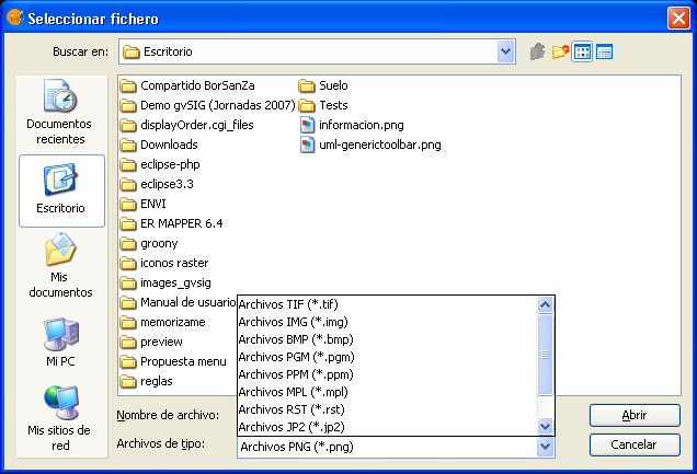
File browser dialog to save the output image
When you select the output file, the Properties button will be enabled.
For example, for geoTiff the dialog will look like this:
Properties geoTiff
- Photometric: [MINISBLACK | MINISWHITE | RGB | CMYK | YCBCR | CIELAB | ICCLAB | ITULAB]. This assigns the photometric interpretation. The default is RGB, as the input image consists of 3 bands of the Byte data type.
- Interleave: [BAND | PIXEL]. By default, tiff files are interleaved by band. Some applications only support interleaved by pixel, in which case you can change this option.
- Compression: [LZW | PACKBITS | DEFLATE | NONE] This refers to the data compression. The default option is NONE.
When the output image is selected and the properties set, you can click on "Apply". A progress bar will appear. Depending on the size of the output file, this process may take while. Processing times may vary between a few seconds or several days, so it is important to check the size of the output image in pixels before clicking "Apply". When finished, a screen with statistics will appear that indicates the path of the output image, the disk size, the duration of the process and whether it was compressed. To check the georeferencing of the output image, you can add it to the view as a new layer with transparency.
Clipping layers
(The clipping tool can be accessed from the raster toolbar by selecting "export to raster" from the left drop-down button and "Clipping" from the drop-down button on the right. Make sure that the raster layer that you want to clip is set as the current layer in the text box.)
With the clipping tool, you can create new layers from an existing one. The options are:
- Extract an area from the input image to be saved as a new layer (cropping)
- Modify the resolution through various interpolation methods
- Modify the order or the number of bands
- Separate the bands into multiple files
Selection of the clipping area
In the "Coordinates" tab of the clipping dialog, there are text boxes to enter coordinates. In the upper part are the values in pixel coordinates and in the lower part the real coordinates. For each item, the two upper text boxes correspond to the coordinates of the upper left corner, while the lower two text boxes correspond to the lower right corner. When changing the pixel coordinates, the real coordinates are re-calculated automatically and vice versa.
There are 3 selection methods that will fill the coordinates automatically. These methods can be activated by clicking the buttons on the bottom of the clipping dialog. From right to left, the buttons are:
- "Select from the view". This is the most commonly used tool to clip a layer. After clicking this button you can draw a rectangle over the view to select the portion of the input layer to be saved as a new layer.
- "Full Extent of the raster layer" When clicking this button, the coordinates of the upper left and lower right corner of the input image are filled in the text boxes.
- "Fit to the maximum extent of the ROIs of the layer". When clicking this button, the extent of the area covered by the ROIs associated with the layer is calculated, and the coordinates are filled in the text boxes.
Clipping dialog. Coordinates tab
Modifying the resolution
In the "Spatial resolution" tab of the Clipping dialog, you can modify the resolution of an output image through various interpolation methods. There are two option boxes located on the upper part of this tab:
- Cell size: Ticking this option will activate the text box labeled "Cell", where you can introduce the new cell size value. By default, the text box shows the cell size of the input image.
- Width x Height: Ticking this option will activate the text boxes labeled "Width" and "Height" where you can introduce the desired width and height of the output image. When changing the width, the height will be re-calculated automatically and vice versa to maintain the correct proportions of the selected area.
When modifying the resolution it is necessary to resample and re-assign the pixel values for the output image through an interpolation method. There are four interpolation methods available: Nearest neighbour, Bilinear, inverse distance and B-Spline. The nearest neighbor is the fastest interpolation method, but the results in pixilation of the image and a lower visual quality. The other interpolation methods produce a smoother result.
The button labeled "Restore" returns the initial values of the input image.
Clipping dialog. Spatial resolution tab
Band selection
The "Bands selection" tab of the Clipping dialog displays a table that lists the bands of the input image. When processed, the output image will have the bands in the order as shown in this list. By default, the output image will have the same order of bands as the input image. The order of the bands can be modified through the "Up" and "Down" buttons. The selected row will go up or down one position in the list. The bands can also be omitted from the resulting image by un-checking the corresponding row.
Clipping dialog. Bands selection tab
Selecting Options
The "Options" tab of the Clipping dialog presents various options that can be set by the user:
- Name of the output layer: you can modify the default name in the textbox labeled "Layer names". This is the name that will appear in the TOC and the name of the file that will be saved to disk. In case of several output layers (i.e. when each band is saved as a separate layer), the name will be the same for each layer but with a number at the end (_XXX). For example, if the layer is called NewLayer and there are 3 output layers, the respective layer names will be NewLayer_1.tif, NewLayer_2.tif and NewLayer_3.tif.
- If the check box labeled as "Create a layer for each band" is ticked, a new layer will be created for each band in the input image.
- If the check box labeled as "Save on disk automatically" is ticked, a text box labeled "Directory" will be activated where you can indicate the file path for the output files. If un-checked, the generated output layers are temporary.
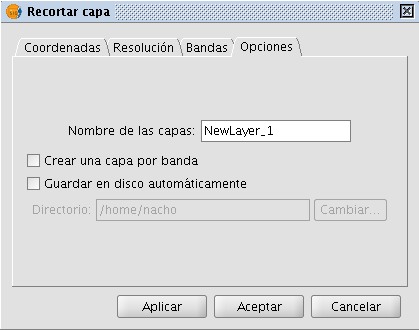
Clipping dialog. Options tab
Zoom to raster resolution
You can zoom to raster resolution by right-clicking on the layer in the TOC. In the context menu that appears, click "Zoom to raster resolution".
This will activate a crosshair cursor in the gvSIG view which allows users to perform an action by clicking somewhere in the view. The action in this case is that with every mouse-click, the view will be centered on the point where you clicked. In addition, the view will zoom so that one screen pixel is the same size as a pixel in the current raster layer.
Automatic vectorization
The "automatic vectorization" function can be launched from the raster toolbar by selecting "Raster process" on the left drop-down button and "Vectorization" on the drop-down button on the right. Make sure that the name of the raster layer that you want to vectorize is displayed as current layer in the text box.

Vectorization icon
With automatic vectorization, you can generate a vector layer from a raster image using preprocessing to highlight the features of interest.
When launching the Vectorization dialog, the first step is to select the area of the image that you want to vectorize. Keep in mind that the vectorization process may take a long time, so it is recommended to minimize the area (number of pixels) for vectorization. The selection of the area for vectorization can be done in several ways. You can type the coordinates directly; either in pixel coordinates or in the map coordinates. The area can also be selected from the view by clicking the button "Select from the view", after which you can draw an approximate rectangle to define the area. Another selection option is by Region Of Interest (ROI). You can define a ROI here or use a previously defined ROI to set the area for vectorization. In the section "ROI selection" appears a list of available ROI and a checkbox next to each of these to select one or more ROI that you want to use. There are two options to vectorize the ROI: to vectorize the entire area inside the rectangle (bounding box) that covers all the selected ROI, or vectorize only the areas inside the ROI while considering the values outside the ROI as NoData values, excluding them from the calculations.
Finally you can select the scale of the image to preprocess. This is useful because a higher resolution of the preprocessed image will result in a higher precision for the resulting vector layer. You can define this with the drop-down text box labelled "Output Scale". By default, the resolution will be the same as the input image.
When moving on to the next step of the wizard, the process of cutting the image for preprocessing is started. A progress bar appears with the warning that this operation could take a few minutes. The resulting image cut is saved in the temporary folder of gvSIG.

Vectorization. Selection of the area to vectorize
There are two methods to preprocess a raster image to vectorize. The first is by creating a limited number of grayscale levels from the original image. The image will be converted to grayscale using one single band or a combination of bands (use the drop-down button labelled "Bands"). For the conversion to grayscale, a posterization process is used to reduce the number of different values. (By default, the image is reduced into 2 levels only: black and white.) For this process you can control the threshold on which the values are passing from black to white and vice versa. This can be done by moving the "Treshold" slider while you can see a preview of the result. (The Treshold slider is only available when there are 2 levels; when there are intermediate grayscale levels, the slider is disabled.) In addition to the posterization threshold, you can apply a mode filter or a noise filter to smoothen the result.

Vectorization. Conversion to grayscale
The second preprocessing method is useful to vectorize contour lines and can be applied to data types other than byte. With this method you can define intervals between each contour line to be vectorized. You can specify the number of intervals in which you want to divide the raster, or indicate the size of each interval. The cuts that have been selected will be shown on a graph that represents the histogram of the image. On this graph, you can modify the distance between cuts, or add or remove some of them using the mouse. It is also possible to modify the distance between cuts in numeric format using the table on the right of the histogram. Each entry in the table represents a cut with the corresponding value. This type of preprocessing is used for digital elevation models (for example .adf or .asc images).
When moving on to the last step of the vectorization wizard, the preprocessed image is generated with the specified values, and saved in the temporary directory of gvSIG.

Vectorization. Define intervals for vectorization in case of Digital Elevation Models
The last step is to select the method for generation of vectors. There are two methods: contour and potrace, that can be selected from the drop-down button after which a panel appears with settings that are specific for the method. The first method is the simplest and does not have any options. This method will trace the vectors in straight sections going through the pixel centers. This generates a network of vectors based on very small straight sections. The potrace method uses the potrace library for vectorization. The available options for this method are those that the potrace library provides and they are used to define the precision of the tracing of the curves: number of points for each curve, threshold, optimization, etc.

Vectorization. Options for vector generation
When clicking on "Apply" or "Accept", the process of vectorization will start after which you will be prompted whether to display the generated layer in the TOC.
Analysis view
The "Analysis view" can be launched from the raster toolbar by selecting "Raster layer" from the left drop-down button and "Analysis View" on the drop-down button on the right. Make sure that the name of the raster layer that you want to analyze is displayed as current layer in the text box.

Analysis View icon
With this functionality you can zoom in on the current raster layer with 3 different zoom levels:
- On the left of the view, the layer is added to the locator map of gvSIG. This provides a general view of the layer, and you can zoom into the locator map by clicking and dragging, thus drawing a red rectangle. The area inside the red rectangle will be displayed in the view.
- The view itself is the second zoom level which functions independently, and the zoom variations that are performed on the view will be applied to the locator map as well so that it keeps being centered on the correct area.
- When launching the Analysis view, a small floating window labelled "Cursor Zoom" appears in the upper right corner of gvSIG. This window has the highest zoom level. The zoom level is fixed and always centered on the mouse point. By moving the mouse over the gvSIG view, you will see the contents change.
You can change the relation between the zoom level of this floating window and the gvSIG view. This is done by right-clicking on the floating window and selecting one of the values that are shown in the drop-down menu that appears. The available options are x4, x8, x16, and x32. This means that the pixels in the floating window will be 4, 8, 16, or 32 times bigger than the original.
The floating window also shows the RGB values of the pixel on which the cursor is currently located. The text colour of the RGB values as well as the colour of the central cross (red by default) can be changed by right-clicking on the floating window and choosing the option from the drop-down menu.
Keep in mind that, to see the effects in the floating window while moving the mouse over the view, the view must be active. If it is not active, just click on the view. When the cursor is outside the view, the content of the floating window appears black.
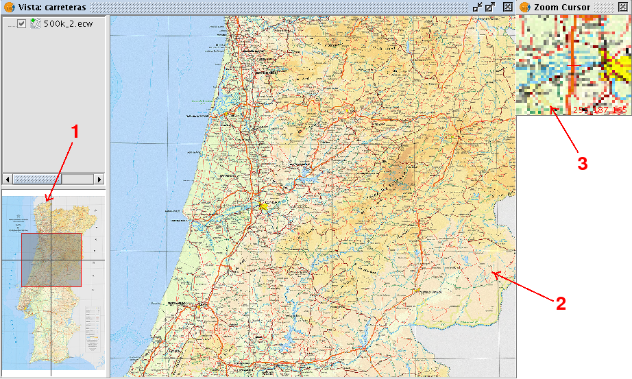
Screenshot with the different elements of Analysis View
There can only be one Analysis view open at any time in gvSIG. Therefore, the button "Analysis View" is re-labelled as "Close Analysis View" when the Analysis view is already open, so that it can be closed before re-opening.
Geographic Transformations
Geolocation
The Geolocation tool provides the ability to change the related transformation that is applied to a raster in its display. A raster could have coordinates that place it in a geographical position. This geographic location is only a change of position, scale and rotation of the image relative to an original position. These changes in position, scale and rotation are those that can be changed with this tool. This can be done numerically and by visual approximation.
This tool does not provide capabilities to deal with complex projections and georeferencing involving the need for resampling.
To launch the geolocation dialogue of the layer, the drop-down toolbar is used by selecting "Geographical Transformations" on the left button and "Geolocation" on the dropdown button on the right. Make sure that the text shows the name of the layer to which we like to assign the transformation.

Geolocation Tool
Upon activating the geolocation tool on a raster layer, a small dialog will appear floating on the view with a series of text entries and a button bar. Also the raster layer that has been selected acquires the capacity to be moved, rotated or moved by clicking and dragging it to the right place on the view.
Transformation on the view
- Translation: When the geolocation tool is active you can move the mouse over the image on the screen and the cursor changes to a hand. This indicates that we can move by clicking and dragging on the raster view.
- Scaling: When the geolocation tool is active you can move the mouse over the edges of the image on screen and the mouse cursor will change. Depending on the chosen edge the cursor will take one form or another. If placed in the top or bottom borders the cursor will become a vertical arrow. This indicates that we can click and drag to scale the image from one side only. The scaling at all times keep the proportions of the raster. If we move the cursor around the side edges the pointer becomes a horizontal arrow now allowing us to scale laterally. In the case of the corners the cursor appears as an oblique arrow.
- Rotation: When the geolocation tool is active, we can move the mouse over the outer corners of the image and the cursor will change. This will appear as a circular arrow. This indicates that we can begin to rotate the raster from the selected corner.
- Shear: When the geolocation tool is active you can move your mouse over the outer side edges of the image and the mouse cursor will change. This will appear as an arrow with a symbol X or Y depending on whether the mouse is in the horizontal or vertical edges respectively. This indicates that we can begin to warp the raster in the direction of the X or the Y.
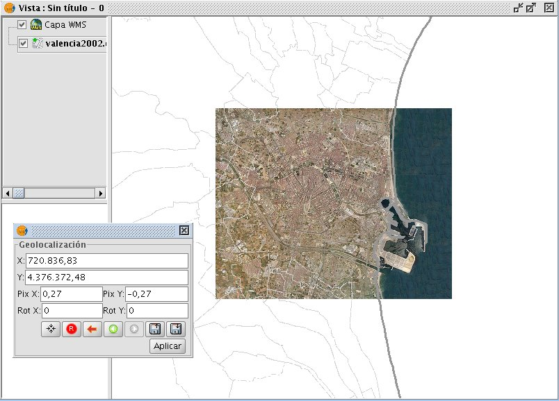
Vista Panel Image Geolocation
Transformation by introducing coordinates
From the geolocation floating box we can modify the transformation of the image on the view. The text entries marked as X, Y, Pix X, Pix Y, Rot X, Rot Y contain the current position in upper left X coordinate, upper left Y coordinate, pixel size in X, pixel size in Y, rotation in X and rotation in Y respectively. If we change these values from the keyboard these will be updated on the image by pressing the "Enter" key while the cursor is inside the text box or when it loses focus.
Controls of the geolocation box
Centering the raster layer in the view: With this button we center the raster in the current view regardless of zoom it has selected. The coordinates will be automatically calculated.
- Initialize the raster transformation: Resets all the transformations that have been applied to the cells back to the default.
- Go to the first processing: Assign the first transformation that was applied.
- Go to the previous transformation: Assign the previous transformation to the current that was applied.
- Go to the next transformation: Assigns the following to the current transformation.
- Upload georeferencing from tfw file: If we have a tfw file with georeferencing coordinates, these can be loaded with this option. A dialog to select the file you want will show up. The extension of the file must be tfw or wld.
- Save current transformation as the default for the raster: Applying this option saves the currently active transformation in the file .rmf attached to raster. Next time the raster is loaded will be with that transformation.
Georeferencing
Description
Direct traslation from Google traslator
To launch the georeferencing dialog it is used the dropdown toolbar selecting the "Geographic Transformations" button on the left and "Georeferencing" from the dropdown button on the right.

Georeferencing Tool
Initially we must decide what type of georeferencing to implement, "reference maps" or "without reference maps".
Georeferencing with "Mapping Reference"
Start Dialogue georeferencing
To implement this type of georeferencing is imperative that we have previously charged in a view mapping that we will provide a geographic reference for taking control points. In case of not having it will close the options dialog georeferencing and proceed to prepare for the hearing. Once we have the view with reference maps georeferencing tool launched will see that the option "reference maps" is checked by default. Below is a dropdown menu which lists the views that gvSIG has at that time. If you have several it must select a view which is our base mapping for decision-points.
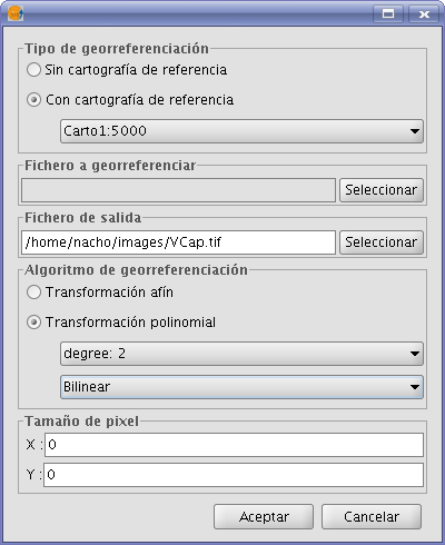
Dialog Georeferencing
In the panel marked "a georeferenced file" pops up a dialog for selecting the file for which you want to create checkpoints and later georeferencing.
The panel labeled "Output File" we must put the path and file name destination if the georeferencing is done with resampling. This option can vary from box options once we are inside the application, so it is not essential to a correct value at the moment, but if must be done before the end of the process.
The panel "georeferencing algorithm" select how we will get the output result. There are two possibilities, "affine transformation" and "polynomial transformation".
The affine transformation applied to raster an affine transformation only to the calculations performed with the control points taken. The affine transformation applied will be allocated "on the fly" for the display and the output image is the same as the input. The result of this transformation is therefore a georeferencing file. Keep in mind that this type of transformation is limited and the user will be responsible for selecting the most convenient transformation in each case.
The polynomial transformation involves a resampling of the input image taking into account the reference control points and obtaining an output image with deformations necessary to adapt to the new location. If you select this option we will be forced to decide the degree of transformation that we apply and the type of interpolation that we want to apply for calculating new pixels. Depending on whether you choose one degree or another need a minimum number of control points for them. This number of points required is given by the formula (order + 1) * (order + 2) / 2, ie for a polynomial of degree one will be needed at least three points, to grade two will need six points for third grade ten points ... The interpolation method affects the way we calculate the information that we have not. When an image georeferenced output image has deformations with respect to the original there are areas where no information is available. These can not be empty with what must be calculated from the areas where we know. These calculations can be performed by various methods, the simplest of these is "Nearest neighbor" which will be unknown pixel information closest known pixel. Other methods such as "bilinear" or "bicubic" make calculations using the known group of pixels surrounding the unknown. These other methods give a more relaxed but it is slower in its implementation. This option can vary from box options once we're inside the application.
The panel "Pixel Pitch" is the pixel size information of the output image. In principle this will be calculated from the input image but can be changed manually. This option can vary from box options once we are inside the application, so it is not essential to a correct value at this time.
The views
Executing the application are two views. The left contains the base mapping that we carry in the gvSIG view of the right and the image we want to georeference. Both have a control bar on the right for view actions. Also in the upper left corner are the coordinates of the mouse cursor. In reference mapping coordinates are those of the real world. In the image to be georeferenced coordinates in pixel coordinate on the upper left.
Cursor Zoom
In the central part appears a cursor with a central window. The window cursor is active when the view can be resized and moved. The contents of this window will be on display in the zoom windows. Ca da vista has its associated zoom window at the bottom. Par resize window cursor select the view you want by clicking on it then bring the mouse to the edges of the window until the pointer changes to horizontal or vertical arrows. Now we click and drag to force the resizing. To move the cursor window select the view you want by clicking on it then bring the mouse to the corners of the window until the pointer changes by crossed arrows. We must now drag and drop to force displacement.
View Controls
There are six controls to handle the zoom level and position of the view mapping Increase the level of zoom: the zoom level increases by multiplying by 2 the current level.

Decrease zoom level: it decreases the zoom level by dividing by 2 the current level.

Zoom area selection: Activates a tool on the hearing in order to make a rectangle the area we want to see enlarged.

Full Zoom: Put a zoom level so that you can view the entire mapping.

Zoom Previous: Sets the zoom level that you previously selected.

Displacement: clicking and dragging on the scroll view mapping.

Zoom controls
Each view has an associated georeferencing zoom window centered over the cursor. When we move the cursor on the sale of view varies the position where the zoom and focus when we change the window size changes the zoom level. In the upper left corner of the window coordinates of the mouse cursor as in the overview.
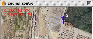
Zoom box associated with the views
Checkpoints
A control point is an entity that provides a correspondence between a geographic coordinate and pixel coordinate. Control points are represented in raster geographic view as Blue-and red circles respectively. To add a new control point is selecting "New" in the table control. This makes a new entry in the table appears. A control point is associated with a table entry. By selecting "New" automatically creates a point at coordinates 0, 0 for both views and will activate the tool "move point". Now clicking on the view point where we will move puncture. We assign the coordinate point numerically by writing directly on the input value in the table (X for the geographic coordinates X, Y geographic coordinate for Y, X 'for X and Y pixel coordinate' for the pixel Y coordinate). The points can also be moved by clicking and dragging on them. This may be done both in hearings and in the zooms.
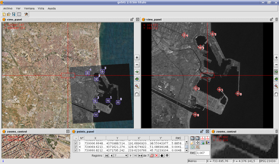
The process of georeferencing. Sights and points of control
Options
The panel labeled "Output File" we must put the path and file name destination if the georeferencing is done with resampling.
The panel georeferencing algorithm "select how we will get the output result. There are two possibilities, "affine transformation" and "polynomial transformation".
The affine transformation applied to raster an affine transformation only to the calculations performed with the control points taken. The affine transformation applied will be allocated on the fly for the display and the output image is the same as the input. The result of this transformation is therefore a georeferencing file. Keep in mind that this type of transformation is limited and the user will be responsible for selecting the most convenient transformation in each case.
The polynomial transformation involves a resampling of the input image taking into account the reference control points and obtaining an output image with deformations necessary to adapt to the new location. If you select this option we will be forced to decide the degree of transformation that we apply and the type of interpolation that we want to apply for calculating new pixels. Depending on whether you choose one degree or another need a minimum number of control points for them. This number of points required is given by the formula (order + 1) * (order + 2) / 2, ie for a polynomial of degree one will be needed at least three points, to grade two will need six points for third grade ten points ... The interpolation method affects the way we calculate the information that we have not. When an image georeferenced output image has deformations with respect to the original there are areas where no information is available. These can not be empty with what must be calculated from the areas where we know. These calculations can be performed by various methods, the simplest of these is "Nearest neighbor" which will be unknown pixel information closest known pixel. Other methods such as "bilinear" or "bicubic" make calculations using the known group of pixels surrounding the unknown. These other methods give a more relaxed but it is slower in its implementation.
The panel "Pixel Pitch" is the pixel size information of the output image. In principle this will be calculated from the input image but can be changed manually.
The panel labeled "Options" contains settings of a different nature. Since we can change the background color of view, the text color of the views. The "show the number of graphically checkpoint" will be displayed or hidden by the control point a point that indicates the corresponding point number. "Add the CSV file errors" will be generated when this type of text files with all the control points we can ignore the file or add the calculated errors. The "Focus the selected point view" makes automatically every time we select a point on the table the view is focused on this. The effect is much as if the tool center point was always active. The "error threshold for the warning," assigns the value at which the error appears in red on the table.
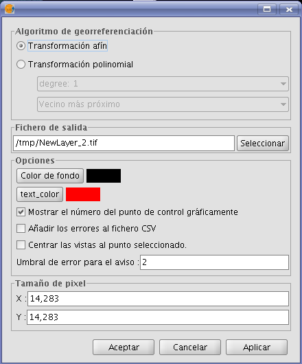
Options for georeferencing
Points Table
The points table is below the sights and initially will be empty. Each table entry corresponds to a checkpoint. It appears all the information related to a point. This table can see it folded its default state or maximized. In its maximized state are folded more information. On the left side of the row there is a check to activate and deactivate the current row. This means that this point will not be displayed graphically or be taken into account for calculation errors and will be prosecuted to do a test. The information can be found in the points table on each point:
- Number of point
- Real coordinate X
- Real coordinate y
- Coordinate pixel X
- Coordinate pixel Y
- Error in X
- Error in Y
- Total RMS error for that point
The quality of the geometric correction can be estimated based on the mean square error RMS error and the contribution of each point. When the contribution to RMS of a point is high, this may indicate that the correspondence of points was poorly selected and the point is not well suited to model transformation between image and map or other information used as reference. The points with high contribution that exceeds a certain threshold can be deleted or deactivated, and calculate the RMS. However, when we are fully confident of the location of a point, and to find you, the RMS is triggered, it may be possible that the geometric model does not resolve the local arrangements, for which they may need a better model, which means, put some more points, right on the problem area.
There is also a global RMS error in an external text field for all points.
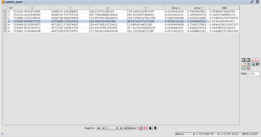
Control Panel points
Controls
Tool center point: When you press the focus control to the view point that is selected.

Georeferencing operation completes. Before you ask if we carry on the gvSIG view the results of the last trial. You'll also want confirmation of application output.

Launching the options dialog.

Make a test with the control points currently entered. If there are not enough for the specified algorithm will warn. The result is that applying the transformation and loading the transformed image on the view with the reference maps.

Save the control points in the metadata file attachment with the raster.

Retrieves the control points that are in the metadata file attached to raster.

Ends the test of processing the raster. Eliminate the test image loaded in the view with the mapping.

When the button "Select point" we are active, clicking on the view assigning the selected point on the table at that time to the position.

Sequence capture control points
There may be ways to capture control points with the tools available. An example would be the following sequence of actions:
- Click "New" in the table of control points. This will create a new row is selected in the table. In addition the tool "Move Point" is selected.
- Click with your mouse pointer over the view to locate the point raster.
- Click with your mouse pointer over the view with reference maps to locate the point.
- Push the button "Refocused selected view point" to place the checkpoint in the center and appears in the zoom window.
- With the tool of choice for area Zoom "or" increase the level of zoom "or" Decrease the zoom level "we can set the desired zoom level until the controls of" Zoom "we have an optimal resolution level approximate.
- Click and drag the control point in the zoom window to place it more precisely. The accuracy depend on how correct is selected previous zoom level.
- Use the zoom tools to return the view to a wider zoom level and to allow a new control point.
- To return to one point and reset the Selection Click on the row of the table, click "Center views the selected point, adjust the zoom level to zoom tools and we'll move the view by clicking and dragging on the window zoom for greater accuracy.
Georeferencing with resampling
Two types of processing for raster. If selected in the options the affine transformation the image obtained is not wide and applies an affine transformation on the view. This transformation is a scaling, displacement, rotation and deformation in the direction of axis X and / or Y axis The transformation with resampling involves generating a new image from the original on which areas can appear empty. These areas are due to the fact that the resulting image should be rectangular but the area covered by the data processing may not have applied this same way.
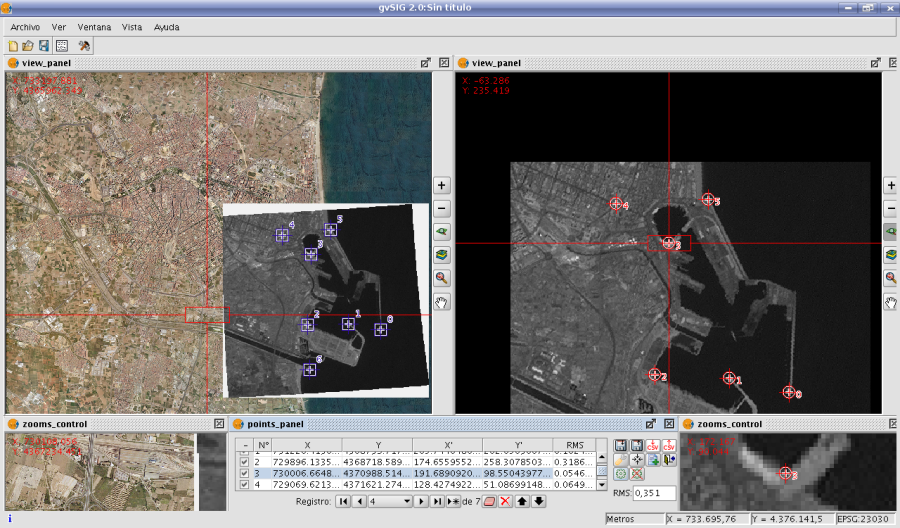
Results georeferenced image with resampling
Once the process of georeferencing the raster generated and loaded in the view we can apply a transparency per pixel to eliminate the empty areas.
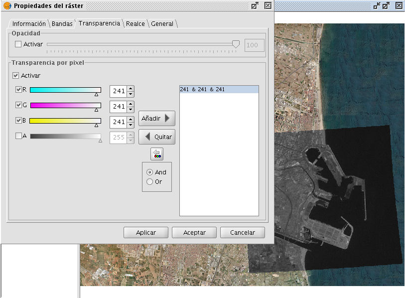
Image georeferenced, with application of transparency
Georeferencing without "Mapping Reference"
The georeferencing without reference maps is useful when you do not have imagery that guide us to assign the control points. We will have to allocate the actual coordinates directly by typing its value. In this case it is useful in view of the left so it will allow more space for the raster and the points table. The operation is very similar to the two views just that when you select the point on the reference maps have to type the entry of the table directly.
The operation of other controls is the same as with reference maps.
Modifying georeferencing upon loading
When you load a file that is not georeferenced, gvSIG can prompt you to enter the coordinates manually. For this the option has to be activated in preferences, which is disabled by default. The option that needs to be activated is "Pedir las coordenadas al cargar un raster que no tiene georreferenciación".
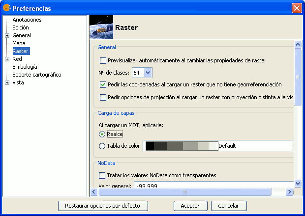
Raster Preferences. Pedir las coordenadas al cargar un raster que no tiene georreferenciación
In this case we will see a dialog with the message: "Name of layer. The layer has no georeferencing. Do you want to enter them manually?". If you answered "No", the load is carried out with the coordinates (0, 0) in the top left corner (width in pixels, height in pixels) in the lower right corner. If the answer is "Yes", then a dialog to enter the coordinates of the raster will show. In this one must be careful to enter valid data to avoid erroneous results. The dialog has two tabs from which we can enter the coordinates in the form of affine transformation or the upper-left and bottom-right corners. In the first mode will need the X and Y coordinates of the upper right corner of the original raster, the pixel size in X, the pixel size on Y, X rotation and the rotation Y.
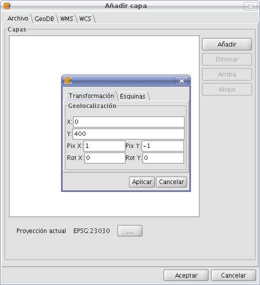
Loading raster without georeference. Transformation
In the second mode we only introduce the coordinates of the corners in the order indicated by the graphs.
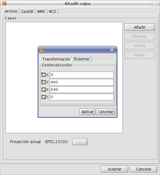
Loading raster without georeference. Corners
Image reprojection
For the reprojection of raster layers, gvSIG uses the GDAL library. The reprojection process can be launched in two different ways: By activating the reprojection icon from the raster toolbar for images that have already been loaded to the view, or by reprojecting the layer before it is loaded to the view if this is needed.
The GDAL library does not support ecw, mrsid or jpeg2000 images and therefore images in these formats cannot be reprojected.
To launch the reprojection dialog from the raster toolbar, select "Geographic transformations" on the left drop-down button and "Reproject layer" on the drop-down button on the right. Make sure that the layer that you want to reproject is set as the current layer in the text box.

Image reprojection icon on the raster toolbar
When launching the reprojection function from the raster toolbar, a dialog opens which shows the projection information of the input image as "source projection". The source projection cannot be changed as it is assumed that the input layer has been loaded into the view with the correct projection. Under "target projection" the projection of the output image can be set by the user through the standard gvSIG dialog for CRS and transformations. It should be noted that not all transformations are supported; the projection options depend on the GDAL reprojection library.
The output layer can be saved on disk or opened in memory as temporary file. When the first option (which is the default) is selected, the user is prompted for a file name and path. Then, the reprojection process starts and when this is finished, it will ask whether you want to add the new layer to the TOC.

Reprojection dialog
NB: When reprojecting an image, the used transformation is "EPSG Transformation"; with raster layers the other transformations (manual, composed or grid) can not be used.
Images can also be reprojected before loading them to the view. To do this, you will need to have the option "Ask for projection when the raster loaded has different projection from view", located in the raster options section of the Preferences dialog, selected. If this option is selected and a raster with a different projection than the view is loaded, a dialog is opened with projection options. The default option is to load the layer while ignoring the projection, but you can reproject the layer by selecting the option "Reproject raster to the view projection". Then, the same Reprojection dialog is shown, but in this case the "target projection" is fixed to the projection of the view, and the "source projection" can be changed, as in some cases the projection of an image may not have been set correctly or the needed projection information maybe missing.
After accepting the settings, the reprojection process will start and the layer will be added to the TOC.

Reprojection options when loading an image to the view
Alphanumeric
Exportar dfb y xls
Exporting Tables to DBF and Excel
The application allows tables (whether layer attribute tables or separate alphanumeric tables ) to be exported in two formats:
- 1.Excel: Export data to a new Microsoft Excel file. The data appears on the second row of the first sheet. The first row contains the column names.
- 2.DBF: Export data to a dBase file.
Follow these steps to export a table:
A. Select the table:
To export a table it must first be opened. The export operations are activated once the table is opened.
To export a subset of the records use the selection tools to select the records to be exported. The records can be selected either from the attribute table or by selecting the corresponding geometries in the View.
B. Select the export option
To do this select the menu option:
For Excel: Table/Export/Excel.
For Dbase: Table/Export/DBF.
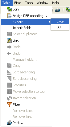
Export to Excel
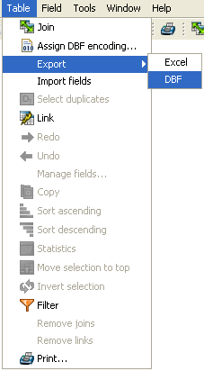
Export to DBF
C. Enter the file name
Locate the directory where you want to create the file and type a name for the file. If the file already exists the application will ask for confirmation to overwrite it.
Unión de Tablas
The tool for joining tables has been improved and now reflects the relationship between the tables once they have been joined. The operation of the tool remains the same in that both tables must contain a common field that will be used to join them together.

Dialog for joining tables
It is possible to add a prefix to the source table fields so that they can be easily identified in the joined table, e.g. Table1_FIELD1, Table1_FIELD2, etc. In a similar manner a prefix can also be added to the target table fields: Table2_FIELD1, Table2_FIELD2, etc.
The resulting joined table is given a title made up of the tables participating in the join, e.g. Table1 X Table2 X, or vice versa.

Result of the table join
The join between the tables can be removed by selecting 'Remove joins' from the Table menu.
- Note: A layer can't be edited once a join has been established on it and the "Start Editing" option on the layer's context menu will be disabled. To start an editing session go to the Table menu and remove the existing joins.
Join
The “Join” tool allows two tables to be joined via a common field. You can also access this tool by clicking on the following button

or by going to the “Table” menu and then to “Join”. To join the two tables, carry out the following steps: Firstly, specify the source table the join is to be made from.
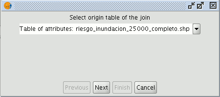
Then specify the field to be used for the join.
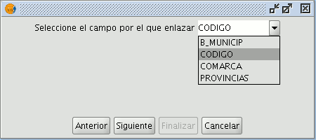
Then indicate the table you wish to join to the first one.
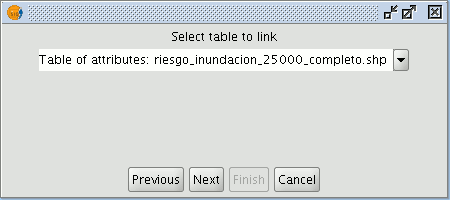
Finally, indicate the field in the second table which is common to the first one.
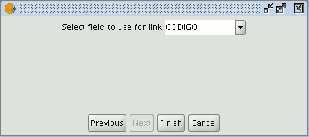
If you open the data source table, you will see that the fields of the destination table have been joined. The name of the field added to the table is identified by the word “Join_(Field name)”
Stadistics
You can access this option by clicking on the following button

or by going to the “Table” menu and then to “Statistics”.
The “Statistics” tool allows you to obtain the most common statistical values.
N.B.: Remember that the tool will not be activated until you select a numerical field.
If you wish to obtain field statistics, select the field (left click on the field heading), then click on the “Statistics” tool.
You can only obtain statistics from a series of records, firstly, select the field the values are located in, then select the desired records, and click on the “Statistics” tool.